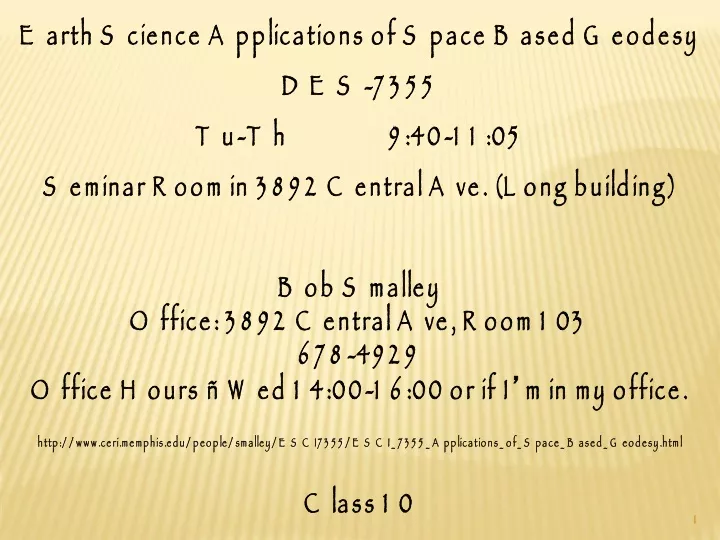
Earth Science Applications of Space Based Geodesy DES-7355 Tu-Th 9:40-11:05

Earth Science Applications of Space Based Geodesy DES-7355 Tu-Th 9:40-11:05 Seminar Room in 3892 Central Ave. (Long building) Bob Smalley Office: 3892 Central Ave, Room 103 678-4929 Office Hours – Wed 14:00-16:00 or if I’m in my office. http://www.ceri.memphis.edu/people/smalley/ESCI7355/ESCI_7355_Applications_of_Space_Based_Geodesy.html Class 10

Using double difference phase observations for relative positioning First notice that if we make all double differences - even ignoring the obvious duplications We get a lot more double differences than original data. This can’t be (can’t create information). Blewitt, Basics of GPS in “Geodetic Applications of GPS”

Consider the case of 3 satellites observed by 2 receivers. Form the (non trivial) double differences Note that we can form any one from a linear combination of the other two (linearly dependent) We need a linearly independent set for Least Squares. Blewitt, Basics of GPS in “Geodetic Applications of GPS”

From the linearly dependent set We can form a number of linearly independent subsets Which we can then use for our Least Squares estimation. Blewitt, Basics of GPS in “Geodetic Applications of GPS”

How to pick the basis? All linearly independent sets are “equally” valid and should produce identical solutions. Pick Ll such that reference satellitel has data at every epoch Better (but harder) approach is to select the reference satellite epoch by epoch (if you have 24 hour data file, cannot pick one satellite and use all day – no satellite is visible all day) Blewitt, Basics of GPS in “Geodetic Applications of GPS”

For a single baseline (2 receivers) that observe s satellites, the number of linearly independent double difference observations is s-1 Blewitt, Basics of GPS in “Geodetic Applications of GPS”

Next suppose we have more than 2 receivers. • We have the same situation • all the double differences are not linearly independent. • As we just did for multiple satellites, we can pick a • reference station • that is common to all the double differences. Blewitt, Basics of GPS in “Geodetic Applications of GPS”

For a network of r receivers, the number of linearly independent double difference observations is r-1 So all together we have a total of (s-1)(r-1) Linearly independent double differences Blewitt, Basics of GPS in “Geodetic Applications of GPS”

So our linearly independent set of double differences is Blewitt, Basics of GPS in “Geodetic Applications of GPS”

Reference station method has problems when all receivers can’t see all satellites at the same time. Choose receiver close to center of network. Blewitt, Basics of GPS in “Geodetic Applications of GPS”

Even this might not work when the stations are very far apart. For large networks may have to pick short baselines that connect the entire network. Idea is to not have any closed polygons (which give multiple paths and are therefore linearly dependent) in the network. Can also pick the reference station epoch per epoch. Blewitt, Basics of GPS in “Geodetic Applications of GPS”

If all the receivers see the same satellites at each epoch, and data weighting is done properly, then it does not matter which receiver and satellite we pick for the reference. Blewitt, Basics of GPS in “Geodetic Applications of GPS”

In practice, however, the solution depends on our choices of reference receiver and satellite. (although the solutions should be similar) (could process all undifferenced phase observatons and estimate clocks at each epoch – ideally gives “better” estimates) Blewitt, Basics of GPS in “Geodetic Applications of GPS”

Double difference observation equations Start with Simplify to By dropping the And assuming are negligible Blewitt, Basics of GPS in “Geodetic Applications of GPS”

Processing double differences between two receivers results in a Baseline solution The estimated parameters include the vector between the two receivers (actually antenna phase centers). May also include estimates of parameters to model troposphere (statistical) and ionosphere (measured – dispersion). Blewitt, Basics of GPS in “Geodetic Applications of GPS”

Also have to estimate the Integer Ambiguities For each set of satellite-receiver double differences Blewitt, Basics of GPS in “Geodetic Applications of GPS”

We are faced with the same task we had before when we used pseudo range We have to linearize the problem in terms of the parameters we want to estimate Blewitt, Basics of GPS in “Geodetic Applications of GPS”

A significant difference between using the pseudo range, which is a stand alone method, and using the Phase, is that the phase is a differential method (similar to VLBI). http://dfs.iis.u-tokyo.ac.jp/~maoxc/its/gps1/node9.html

So far we have cast the problem in terms of the distances to the satellites, but we could recast it in terms of the relative distances between stations. http://dfs.iis.u-tokyo.ac.jp/~maoxc/its/gps1/node9.html

So now we will need multiple receivers. We will also have to use (at least one) as a reference station. In addition to knowing where the satellites are, We need to know the position of the refrence station(s) to the same level of precision as we wish to estimate the position of the other stations. http://dfs.iis.u-tokyo.ac.jp/~maoxc/its/gps1/node9.html

fiducial positioning Fiducial Regarded or employed as a standard of reference, as in surveying. http://dictionary.reference.com/search?q=fiducial

So now we have to assign the location of our fiducial station(s) Can do this with RINEX header position VLBI position Other GPS processing etc. http://dictionary.reference.com/search?q=fiducial

So we have to Write down the equations Linearize Solve Blewitt, Basics of GPS in “Geodetic Applications of GPS”

Double difference observation equations Start with Simplify to By dropping the And assuming are negligible Blewitt, Basics of GPS in “Geodetic Applications of GPS”

So we have to Write down the equations Linearize Solve Blewitt, Basics of GPS in “Geodetic Applications of GPS”

Let the “reference” (also KNOWN) station be A We want to estimate (xB,yB,zB) Using observations of satellites 1, 2, 3, and 4 (common observations at all epochs) We also need to pick a “reference” satellite (position of all satellites known) Pick satellite 2. (we have to pick the reference station and satellite to properly form a linearly independent set of double differences) Blewitt, Basics of GPS in “Geodetic Applications of GPS”

For each epoch i We have the following 3 linearly independent sets of double difference observations To estimate the parameter set (if there were no cycle slips, else we would have to estimate additional NABij(k) term for each cycle slip, k. Blewitt, Basics of GPS in “Geodetic Applications of GPS”

As before, the linearized observation equations can be written in terms of the “usual suspects” Residuals – d x 1 Observation errors – d x 1 “design” matrix - d x p Parameter corrections – p x 1 d – number linearly independent observables p – number of parameters to estimate Blewitt, Basics of GPS in “Geodetic Applications of GPS”

In comparison to the pseudo range data, where we assumed the errors in the observables were independent, the errors in double differenced data are not – the errors are correlated. This means that we should use Weighted Least Squares Blewitt, Basics of GPS in “Geodetic Applications of GPS”

The WLS solution to the normal equations is Where W is (an appropriately formed) data weight matrix. The covariance matrix is now given by (does this look familiar?) Blewitt, Basics of GPS in “Geodetic Applications of GPS”

The covariance matrix now has information about both the geometry (as before) And new (information or effects due to) correlations between the observables. (if we assume, as for pseudo range, that the error in measurement of the phase is the same for all measurements – we can factor out a s, But the differencing introduces a correlation between the “independent” measurements that makes the errors “leak” from one observable to another)

Again, one can get important information from the Covariance matrix If it is not invertable mathematically (linearly dependent) If it is not invertable practically/numerically (almost linearly dependent, large condition number) Practically, can tell if all the integer ambiguities can be fixed. If so, get statistically better estimations. Blewitt, Basics of GPS in “Geodetic Applications of GPS”

Coefficients of the design matrix Look at one row. Blewitt, Basics of GPS in “Geodetic Applications of GPS”

Coefficients of the design matrix Look at one derivative. Independent of xB Blewitt, Basics of GPS in “Geodetic Applications of GPS”

Coefficients of the design matrix Finally one can use the relationship between Range and Time and Time and Phase (what we measured). To write everything in terms of the observables. Blewitt, Basics of GPS in “Geodetic Applications of GPS”

Final detail Minimum data requirements Necessary (but not sufficient condition) that Number of data Exceed Number of parameters to estimate. Blewitt, Basics of GPS in “Geodetic Applications of GPS”

So we have d≥p (allowing perfect solution d=p) If all receivers track the same satellites there are d=q(r-1)(s-1) Linearly independent double differences Where q is the number of epochs r the number of receivers s the number of satellites Blewitt, Basics of GPS in “Geodetic Applications of GPS”

Assuming no cycle slips p=3+(r-1)(s-1) So d=q(r-1)(s-1)≥ 3+(r-1)(s-1) (q-1)(r-1)(s-1)≥ 3 So for r=2, s=2 q≥4 (gives one double difference per epoch) Blewitt, Basics of GPS in “Geodetic Applications of GPS”

Common-mode Cancellations After Glen Mattioli

RINEX files Receiver Independent Exchange files (standard GPS, now GNSS, observables – data – file) ASCII files (text – you can read them) New competitor – may replace RINEX – BINEX Binary Exchange files (binary – can’t read files without program, much more general == complicated)

RINEX Files have two basic parts Header Data (observables)

RINEX Header +--------------------+------------------------------------------+------------+*|INTERVAL | Observation interval in seconds | F10.3 |* +--------------------+------------------------------------------+------------+ |TIME OF FIRST OBS | - Time of first observation record | 5I6,F13.7, | | | (4-digit-year, month,day,hour,min,sec) | | | | - Time system: GPS (=GPS time system) | 5X,A3 | | | GLO (=UTC time system) | | | | Compulsory in mixed GPS/GLONASS files | | | | Defaults: GPS for pure GPS files | | | | GLO for pure GLONASS files | | +--------------------+------------------------------------------+------------+*|TIME OF LAST OBS | - Time of last observation record | 5I6,F13.7, |* | | (4-digit-year, month,day,hour,min,sec) | | | | - Time system: Same value as in | 5X,A3 || | | TIME OF FIRST OBS record | || +--------------------+------------------------------------------+------------+*|RCV CLOCK OFFS APPL | Epoch, code, and phase are corrected by | I6 |* | | applying the realtime-derived receiver | | | | clock offset: 1=yes, 0=no; default: 0=no | | | | Record required if clock offsets are | | | | reported in the EPOCH/SAT records | | +--------------------+------------------------------------------+------------+*|LEAP SECONDS | Number of leap seconds since 6-Jan-1980 | I6 |* | | Recommended for mixed GPS/GLONASS files | | +--------------------+------------------------------------------+------------+*|# OF SATELLITES | Number of satellites, for which | I6 |* | | observations are stored in the file | |

Header example 2.10OBSERVATION DATA M (MIXED) RINEX VERSION / TYPEBLANK OR G = GPS, R = GLONASS, T = TRANSIT, M = MIXED COMMENTXXRINEXO V9.9 AIUB 24-MAR-01 14:43 PGM / RUN BY / DATEEXAMPLE OF A MIXED RINEX FILE COMMENTA 9080 MARKER NAME9080.1.34 MARKER NUMBERBILL SMITH ABC INSTITUTE OBSERVER / AGENCYX1234A123 XX ZZZ REC # / TYPE / VERS234 YY ANT # / TYPE4375274. 587466. 4589095. APPROX POSITION XYZ.9030 .0000 .0000 ANTENNA: DELTA H/E/N 1 1 WAVELENGTH FACT L1/2 1 2 6 G14 G15 G16 G17 G18 G19 WAVELENGTH FACT L1/2 0 RCV CLOCK OFFS APPL 4 P1 L1 L2 P2 # / TYPES OF OBSERV 18.000 INTERVAL 2001 3 24 13 10 36.0000000 TIME OF FIRST OBS END OF HEADER (I’ve not seen many headers with the “time of last observation” line)

Another header example 2.10 OBSERVATION DATA G (GPS) RINEX VERSION / TYPE teqc 2005Feb10 You don't know? 20050411 15:07:57UTCPGM / RUN BY / DATE Linux 2.0.36|Pentium II|gcc|Linux|486/DX+ COMMENT BIT 2 OF LLIGFLAGS DATA COLLECTED UNDER A/S CONDITION COMMENT CJTR MARKER NAME -Unknown- -Unknown- OBSERVER / A ENCY 664 ASHTECH Z-12 CD00 REC # / TYPE / VERS 943 -Unknown- ANT # / TYPE 0.0000 0.0000 0.0000 APPROX POSITION XYZ 0.0000 0.0000 0.0000 ANTENNA: DELTA H/E/N 1 1 WAVELENGTH FACT L1/2 5 L1 L2 C1 P1 P2 # / TYPES OF OBSERV SNR is mapped to RINEX snr flag value [0-9] COMMENT L1 & L2: 2-19 dBHz = 1, 20-27 dBHz = 2, 28-31 dBHz = 3 COMMENT 32-35 dBHz = 4, 36-38 dBHz = 5, 39-41 dBHz = 6 COMMENT 42-44 dBHz = 7, 45-48 dBHz = 8, >= 49 dBHz = 9 COMMENT pseudorange smoothing corrections not applied COMMENT 2004 12 26 0 0 30.0000000 TIME OF FIRST OBS END OF HEADER Not having an X0 estimate makes processing more difficult

Earth Science Applications of Space Based Geodesy DES-7355 Tu-Th 9:40-11:05