Download
1 / 22
290 likes | 549 Views
Introduction to Econometrics. Week 4 Multiple regression models. Lecture plan. the need for additional regressors classical assumptions and least squares estimation extended to allow for several regressors interpreting the results t tests of individual parameter values

E N D
Introduction to Econometrics Week 4 Multiple regression models
Lecture plan • the need for additional regressors • classical assumptions and least squares estimation extended to allow for several regressors • interpreting the results • t tests of individual parameter values • R squared and R bar squared • Analysis of variance and F tests • practical illustrations
multiple regression models: examples • sales-advertising equations may need to be extended to include variables such as consumers income, price and the price and advertising of competitors’ products • earnings equations may need to be extended to include experience or age and other variables in addition to years of schooling (including dummyvariables to examine the importance of gender, ethnic group etc.)
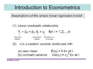
Assumptions of the multiple linear regression model (1) A stable linear stochastic relationship • Yi = b0 + b1 X1i + b2 X2i +....+ bk Xki + ui • for i = 1,2,...,n The parameters are the same for each observation – no structural differences
Assumptions of the multiple linear regression model (2) u is a random variable distributed with (a) zero mean E(ui) = 0 for all i (b) constant variance var(ui) = su2 for all i (b) implies disturbances are “homoskedastic”
Assumptions of the multiple linear regression model (3) Disturbances are independent of one another E(ui|uj ) = 0 for i j Note: independence means E(ui|uj ) = E(ui ) which = 0 by assumption 2a
Assumptions of the multiple linear regression model (4) Disturbances are independent of each of the X variables E(ui|Xj) = E(ui) = 0 for all i, j
Assumptions of the multiple linear regression model (5) u has a normal distribution thus with (2) we can write u ~ N(0, su2)
Assumptions of the multiple linear regression model (6) There is no exact linear relationship among the X variables (they are linearly independent)
A regression plane rather than a regression line For the case of two independent variables we fit a regression plane through a scatter of points in 3 dimensional space
Tests of significance of the individual parameter estimates (1)
Tests of significance of the individual parameter estimates (2)
Testing the overall significance of the regression. Analysis of variance (F test)
R squared and the F value It is also possible to calculate an F value from the value of R squared
more on the extended sales model sales = b0+b1price+b2income+b3pcompet+b4ads + u
more on the extended earnings model earnings = b1+b2s+b3exper + u