Introduction to Econometrics

1. Econometrics I Summer 2011/2012 Course Guarantor:  prof. Ing. Zlata Sojková, CSc., Lecturer: Ing. Martina Hanová, PhD. Introduction to Econometrics

2. „Econometrics may be defined as the social science in which the tools of economic theory, mathematics, and statistical inference are applied to the analysis of economic phenomena.“ (Arthur S. Goldberger) Econometrics

3. Econometrics Statistics Mathematics Economics Econometrics - uses a variety of techniques, including regression analysis to compare and test two or more variables. Econometrics is a mixture of economic theory, mathematical economics, economic statistics, and mathematical statistics. Econometric Theory

4. Traditional or classical methodology 1. Statement of theory or hypothesis 2. Specification of the mathematical model 3. Specification of the statistical, or econometric model 4. Obtaining the data 5. Estimation of the parameters of the econometric model 6. Hypothesis testing 7. Forecasting or prediction 8. Using the model for control or policy purposes. Methodology of Econometrics

5. A theory should have a prediction – hypothesis (in statistics and econometrics) Keynesian theory of consumption: Keynes stated - men are disposed to increase their consumption as their income increases, but not as much as the increase in their income. marginal propensity to consume (MPC) - is greater than zero but less than 1. 1. Theory or hypothesis

6. Mathematical equation: Y = β1 + β2X β1 intercept and β2 a slope coefficient. Keynesian consumption function: Y = consumption expenditure X = income β2 measures the MPC 0 < β2 < 1 2. Mathematical Model

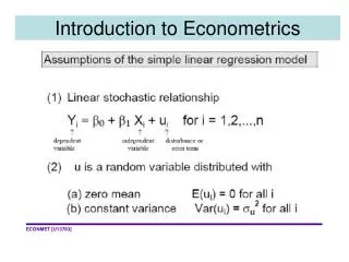
7. Mathematical model- deterministic relationship between variables Econometric model – random or stochastic relationship between variables Y = β1 + β2X + u Y = β1 + β2X +  u or - disturbance,error term, or random (stochastic) variable - represents other non-quantifiable, unknown factors that affect Y. • measurement errors • reporting errors • computing errors • other influence, 3. Specification of the Econometric Model

8. 4. Obtain Data • observational data non-experimental data, • experimental data Types of Data • time series data • cross-section data • pooled data Measurement of Scale • Ratio scale • Interval scale • Ordinal scale • Nominal scale

9. to estimate the parameters of the function, β1 and β2, Statistical technique - regression analysis Ŷ= −184.08 + 0.7064X Ŷ - is an estimate of consumption 5. Estimation of the model

10. 6. Hypothesis Testing statistical inference (hypothesis testing) 7. Forecasting forecast, variable Y on the basis of known or expected future value(s) of the explanatory, or predictor, variable X. 8. Use for Policy Recommendation

11. TERMINOLOGY AND NOTATION • Dependent variable • Explained variable • Predictand • Regressand • Response • Endogenous • Outcome • Controlled variable • Independent variable • Explanatory variable • Predictor • Regressor • Stimulus • Exogenous • Covariate • Control variable • two-variable (simple) regression analysis • multiple regression analysis • multivariate regression vs. multiple regression

12. Method of Least Squares (MLS) A. Theory B. Estimation of parameters Ordinary Least Squares (OLS)

13. E(YiXi) = o + 1Xi population regression line (PRF) • Ŷi= bo + b1Xi sample regression equation (SRF) min  ei2 = e12 + e22 + e32 +.........+ en2 The Theoryof OLS

14. Excel Tools/data analysis/ regression Matrix form Formula – mathematical function How does OLS get estimates of the coefficients?