Download
1 / 21
210 likes | 514 Views
Distance-based methods. Xuhua Xia xxia@uottawa.ca http://dambe.bio.uottawa.ca. Lecture Outline. Objectives in this lecture Grasp the basic concepts distance-based tree-building algorithms

E N D
Distance-based methods Xuhua Xia xxia@uottawa.ca http://dambe.bio.uottawa.ca
Lecture Outline • Objectives in this lecture • Grasp the basic concepts distance-based tree-building algorithms • Learn the least-squares criterion and the minimum evolution criterion and how to use them to construct a tree • Distance-based methods • Genetic distance: generally defined as the number of substitutions per site. • JC69 distance • K80 distance • TN84 distance • F84 distance • TN93 distance • LogDet distance • Tree-building algorithms (UPGMA): • UPGMA • Neighbor-joining • Fitch-Margoliash • FastME Slide 2
Genetic Distances • Genetic distances: Assuming a substitution model, we can obtain the genetic distance (i.e., difference) between two nucleotide or amino acid sequences, e.g., • JC • K80 • TN93: Slide 3
Calculation of KJC69 AACGACGATCG: Species 1 AACGACGATCG AACGACGATCG: Species 2 t t The time is 2t between Species 1 to Species 2 Sp1: AAG CCT CGG GGC CCT TAT TTT TTG || | ||| ||| | ||| ||| || Sp2: AAT CTC CGG GGC CTC TAT TTT TTT p = 6/24 = 0.25 K = 0.304099 Genetic distances are scaled to be the number of substitutions per site. Slide 4
Numerical Illustration Sp1: AAG CCT CGG GGC CCT TAT TTT TTG || | ||| ||| | ||| ||| || Sp2: AAT CTC CGG GGC CTC TAT TTT TTT What are P and Q? P = 4/24, Q = 2/24 Comparison of distances: P = 0.25 Poisson P = -ln(1-p) = 0.288 KJC69 = 0.304099 KK80 = 0.3150786 Slide 5
A Star Tree (Completely Unresolved Tree) Human Chimpanzee Gorilla Orangutan Gibbon Slide 7
Genetic Distance Matrix Matrix of Genetic distances (Dij): Human Chimp Gorilla Orang GibbonHuman 0.015 0.045 0.143 0.198Chimp 0.030 0.126 0.179Gorilla 0.092 0.179Orang 0.179Gibbon Slide 8
UPGMA • Human Chimp Gorilla Orang GibbonHuman 0.015 0.045 0.143 0.198Chimp 0.030 0.126 0.179Gorilla 0.092 0.179Orang 0.179Gibbon • D(hu-ch),go = (Dhu,go + Dch,go)/2 = 0.038 D(hu-ch),or = (Dhu,or + Dch,or)/2 = 0.135D(hu-ch),gi = (Dhu,gi + Dch,gi)/2 = 0.189 • hu-ch Gorilla Orang Gibbonhu-ch 0.038 0.135 0.189Gorilla 0.092 0.179Orang 0.179Gibbon Human Chimp Gorilla Orang Gibbon Gorilla Orang Gibbon Human Chimp (hu,ch),(go,or,gi) Orang Gibbon Gorilla Human Chimp ((hu,ch),go),(or,gi) Slide 9
UPGMA • Human Chimp Gorilla Orang GibbonHuman 0.015 0.045 0.143 0.198Chimp 0.030 0.126 0.179Gorilla 0.092 0.179Orang 0.179Gibbon • D(hu-ch-go),or = (Dhu,or + Dch,or + Dgo,or)/3 = 0.120D(hu-ch-go),gi = (Dhu,gi + Dch,gi +Dgo,gi)/3 = 0.185 • hu-ch-go Orang Gibbonhu-ch-go 0.120 0.185Orangutan 0.179Gibbon • D(hu-ch-go-or),gi = (Dhu,gi + Dch,gi +Dgo,gi + Dor,gi)/4 = 0.184 Orang Gibbon Gorilla Human Chimp Gibbon Orang Gorilla Human Chimp (((hu,ch),go),or),gi) Slide 10
Phylogenetic Relationship from UPGMA • Human Chimp Gorilla Orang GibbonHuman 0.015 0.045 0.143 0.198Chimp 0.030 0.126 0.179Gorilla 0.092 0.179Orang 0.179Gibbon • hu-ch Gorilla Orang Gibbonhu-ch 0.038 0.135 0.189Gorilla 0.092 0.179Orang 0.179Gibbon • hu-ch-go Orang Gibbonhu-ch-go 0.120 0.185Orang 0.179Gibbon Slide 11
Branch Lengths ((hu,ch),(go,or,gi)) (((hu,ch),go),(or,gi)) ((((hu,ch),go),or),gi) Dhu-ch = 0.015 D(hu-ch),go = (Dhu,go + Dch,go)/2 = 0.038 D(hu-ch),or = (Dhu,or + Dch,or)/2 = 0.135D(hu-ch),gi = (Dhu,gi + Dch,gi)/2 = 0.189 D(hu-ch-go),or = (Dhu,or + Dch,or + Dgo,or)/3 = 0.120D(hu-ch-go),gi = (Dhu,gi + Dch,gi +Dgo,gi)/3 = 0.185 D(hu-ch-go-or),gi = (Dhu,gi + Dch,gi +Dgo,gi + Dor,gi)/4 = 0.184 0.0075 Human Chimp Gorilla Orang Gibbon 0.019 0.06 ((hu:0.0075,ch:0.0075),(go,or,gi)) (((hu:0.0075,ch:0.0075):0.019,go:0.019),(or,gi)) ((((hu:0.0075,ch:0.0075):0.0115,go:0.019):0.041,or:0.06):0.032,gi:0.092) 0.092 Slide 12
Final UPGMA Tree Human Chimp Gorilla Orang Gibbon 19 13 8 6 MY 0.092 0.060 0.019 0.0075 ((((hu:0.0075,ch:0.0075):0.0115,go:0.019):0.041,or:0.06):0.032,gi:0.092); Slide 13
Distance-based method • Distance matrix • Tree-building algorithms • UPGMA • Neighbor-joining • FastME • Fitch-Margoliash • Criterion-based methods • Branch-length estimation • Tree-selection criterion Slide 14
Branch Length Estimation • For three OTUs, the branch lengths can be estimated directly • For more than three OTUs, there are two commonly used methods for estimating branch lengths • The least-square method • Fitch-Margoliash method • Don’t confuse the Fitch-Margoliash method of branch length estimation with the Fitch-Margoliash criterion of tree selection • Illustration of the least-square method of branch length estimation Slide 15
For three OTUs 1 x1 x3 3 x2 2 1 2 3 1 0.092 0.1792 0.1793 1 2 31 d12 d132 d233 d12 = x1 + x2 d13 = x1 + x3 d23 = x2 + x3 Slide 16
Least-square method 1 3 x3 x1 x5 x2 x4 2 4 4 Sp1 Sp2 0.3 Sp3 0.4 0.5 Sp4 0.4 0.6 0.6 4 Sp1 Sp2 d12 Sp3 d13 d23 Sp4 d14 d24 d34 Slide 17
Least-square method 1 3 x3 x1 x5 Least-squares method: Find xi values that minimize SS x2 x4 2 4 d’12 = x1 + x2 d’13 = x1 + x5+ x3 d’14 = x1 + x5 + x4 d’23 = x2 + x5 + x3 d’24 = x2 + x5 + x4 d’34 = x3 + x4 (d12 - d’12)2= [d12 – (x1 + x2)]2 (d13 - d’13)2 = [d13 – (x1 + x5+ x3)]2 (d14 - d’14)2 = [d14 – (x1 + x5 + x4)]2 (d23 - d’23)2 = [d23 – (x2 + x5 + x3)]2 (d24 - d’24)2 = [d24 – (x2 + x5 + x4)]2 (d34 - d’34)2 = [d34 – (x3 + x4)]2 Slide 18
Least-squares method SS = [d12 – (x1 + x2)]2 + [d13 – (x1 + x5+ x3)]2 + [d14 – (x1 + x5 + x4)]2 + [d23 – (x2 + x5 + x3)]2+ [d24 – (x2 + x5 + x4)]2+ [d34 – (x3 + x4)]2 Take the partial derivative of SS with respective to xi, we have SS/x1 := -2 d12 + 6 x1 + 2 x2 - 2 d13 + 4 x5 + 2 x3 - 2 d14 + 2 x4 SS/x2 := -2 d12 + 2 x1 + 6 x2 - 2 d23 + 4 x5 + 2 x3 - 2 d24 + 2 x4 SS/x3 := -2 d13 + 2 x1 + 4 x5 + 6 x3 - 2 d23 + 2 x2 - 2 d34 + 2 x4 SS/x4 := -2 d14 + 2 x1 + 4 x5 + 6 x4 - 2 d24 + 2 x2 - 2 d34 + 2 x3 SS/x5 := -2 d13 + 4 x1 + 8 x5 + 4 x3 - 2 d14 + 4 x4 - 2 d23 + 4 x2 - 2 d24 Setting these partial derivatives to 0 and solve for xi, we have x1 = d13/4 + d12/2 - d23/4 + d14/4 - d24/4 x2 = d12/2 - d13/4 + d23/4 - d14/4 + d24/4, x3 = d13/4 + d23/4 + d34/2 - d14/4 - d24/4, x4 = d14/4 - d13/4 - d23/4 + d34/2 + d24/4, x5 = - d12/2 + d23/4 - d34/2 + d14/4 + d24/4 + d13/4 Slide 19
Least-squares method 1 3 x3 x1 x5 x2 x4 2 4 x1 = d13/4 + d12/2 - d23/4 + d14/4 - d24/4 x2 = d12/2 - d13/4 + d23/4 - d14/4 + d24/4, x3 = d13/4 + d23/4 + d34/2 - d14/4 - d24/4, x4 = d14/4 - d13/4 - d23/4 + d34/2 + d24/4, x5 = - d12/2 + d23/4 - d34/2 + d14/4 + d24/4 + d13/4 4 Sp1 Sp2 0.3 Sp3 0.4 0.5 Sp4 0.4 0.6 0.6 x1 = 0.075 x2 = 0.225 x3 = 0.275 x4 = 0.325 x5 = 0.025 Slide 20
Minimum Evolution Criterion 1 1 1 2 2 3 x3 x3 x3 x1 x1 x1 x5 x5 x5 x2 x2 x2 x4 x4 x4 4 2 3 4 4 3 The minimum evolution (ME) criterion: The tree with the shortest TreeLen is the best tree. Slide 21