Download
1 / 41
450 likes | 866 Views
Distance Matrix Methods. Anders Gorm Pedersen Molecular Evolution Group Center for Biological Sequence Analysis Technical University of Denmark gorm@cbs.dtu.dk. Distance Matrix Methods. Construct multiple alignment of sequences

E N D
Distance Matrix Methods Anders Gorm Pedersen Molecular Evolution Group Center for Biological Sequence Analysis Technical University of Denmark gorm@cbs.dtu.dk
Distance Matrix Methods • Construct multiple alignment of sequences • Construct table listing all pairwise differences (distance matrix) • Construct tree from pairwise distances Gorilla : ACGTCGTA Human : ACGTTCCT Chimpanzee: ACGTTTCG Ch 1 1 1 Hu 2 Go
Finding optimal branch lengths S2 S1 a c b e d S3 S4 Distance along tree (patristic distance) Observed distance D12 d12 = a + b + c D13 d13 = a + d D14 d14 = a + b + e D23 d23 = d + b + c D24 d24 = c + e D34 d34 = d + b + e Goal:
Exercise (handout) • Construct distance matrix (count different positions) • Reconstruct tree and find best set of branch lengths
Optimal Branch Lengths for a Given Tree: Least Squares • Fit between given tree and observed distances can be expressed as “sum of squared differences”: Q = (Dij - dij)2 • Find branch lengths that minimize Q - this is the optimal set of branch lengths for this tree. S2 S1 a c b e d S3 S4 Distance along tree j>i D12 d12 = a + b + c D13 d13 = a + d D14 d14 = a + b + e D23 d23 = d + b + c D24 d24 = c + e D34 d34 = d + b + e Goal:
Optimal Branch Lengths: Least Squares • Longer distances associated with larger errors • Squared deviation may be weighted so longer branches contribute less to Q: Q = (Dij - dij)2 • Power (n) is typically 1 or 2 S2 S1 a c b e d S3 S4 Distance along tree D12 d12 = a + b + c D13 d13 = a + d D14 d14 = a + b + e D23 d23 = d + b + c D24 d24 = c + e D34 d34 = d + b + e Dijn Goal:
Finding Optimal Branch Lengths A v1 v3 C v2 B Observed distance Distance along tree DAB dAB = v1 + v2 DAC dAC = v1 + v3 DBC dBC = v2 + v3 Goal:
Finding Optimal Branch Lengths • System of n linear equations with n unknowns • Can be solved using substitution method or matrix-based methods
Least Squares Optimality Criterion • Search through all (or many) tree topologies • For each investigated tree, find best branch lengths using least squares criterion • Among all investigated trees, the best tree is the one with the smallest sum of squared errors. • Least squares criterion used both for finding branch lengths on individual trees, and for finding best tree.
Minimum Evolution Optimality Criterion • Search through all (or many) tree topologies • For each investigated tree, find best branch lengths using least squares criterion • Among all investigated trees, the best tree is the one with the smallest sum of branch lengths (the shortest tree). • Least squares criterion used for finding branch lengths on individual trees, minimum tree length used for finding best tree.
Superimposed Substitutions • Actual number of evolutionary events: 5 • Observed number of differences: 2 • Distance is (almost) always underestimated ACGGTGC C T GCGGTGA
Model-based correction for superimposed substitutions • Goal: try to infer the real number of evolutionary events (the real distance) based on • Observed data (sequence alignment) • A model of how evolution occurs
Jukes and Cantor Model • Four nucleotides assumed to be equally frequent (f=0.25) • All 12 substitution rates assumed to be equal • Under this model the corrected distance is: DJC = -0.75 x ln(1-1.33 x DOBS) • For instance: DOBS=0.43 => DJC=0.64
Clustering Algorithms • Starting point: Distance matrix • Cluster least different pair of nodes: • Tree: connect pair of nodes to common ancestral node, compute branch lengths from ancestral node to both descendants • Distance matrix: combine two entries into one. Compute new distance matrix, by finding distance from new node to all other nodes • Repeat until all nodes are linked • Results in only one tree, there is no measure of tree-goodness.
Neighbor Joining Algorithm • For each tip compute ui = jDij/(n-2) (this is essentially the average distance to all other tips, except the denominator is n-2 instead of n) • Find the pair of tips, i and j, where Dij-ui-uj is smallest • Connect the tips i and j, forming a new ancestral node. The branch lengths from the ancestral node to i and j are: vi = 0.5 Dij + 0.5 (ui-uj) vj = 0.5 Dij + 0.5 (uj-ui) • Update the distance matrix: Compute distance between new node and each remaining tip as follows: Dij,k = (Dik+Djk-Dij)/2 • Replace tips i and j by the new node which is now treated as a tip • Repeat until only two nodes remain.
Neighbor Joining Algorithm Dij-ui-uj
Neighbor Joining Algorithm Dij-ui-uj
Neighbor Joining Algorithm C D X Dij-ui-uj
Neighbor Joining Algorithm C D 10 4 X vC = 0.5 x 14 + 0.5 x (23.5-29.5) = 4 vD = 0.5 x 14 + 0.5 x (29.5-23.5) = 10 Dij-ui-uj
Neighbor Joining Algorithm C D 10 4 X
Neighbor Joining Algorithm DXA = (DCA + DDA - DCD)/2 = (21 + 27 - 14)/2 = 17 DXB = (DCB + DDB - DCD)/2 = (12 + 18 - 14)/2 = 8 C D 10 4 X
Neighbor Joining Algorithm DXA = (DCA + DDA - DCD)/2 = (21 + 27 - 14)/2 = 17 DXB = (DCB + DDB - DCD)/2 = (12 + 18 - 14)/2 = 8 C D 10 4 X
Neighbor Joining Algorithm DXA = (DCA + DDA - DCD)/2 = (21 + 27 - 14)/2 = 17 DXB = (DCB + DDB - DCD)/2 = (12 + 18 - 14)/2 = 8 C D 10 4 X
Neighbor Joining Algorithm C D 10 4 X
Neighbor Joining Algorithm C D 10 4 X Dij-ui-uj
Neighbor Joining Algorithm C D 10 4 X Dij-ui-uj
Neighbor Joining Algorithm C A D B 4 10 13 4 X Y vA = 0.5 x 17 + 0.5 x (34-25) = 13 vD = 0.5 x 17 + 0.5 x (25-34) = 4 Dij-ui-uj
Neighbor Joining Algorithm C A D B 4 10 13 4 X Y
Neighbor Joining Algorithm DYX = (DAX + DBX - DAB)/2 = (17 + 8 - 17)/2 = 4 C A D B 4 10 13 4 X Y
Neighbor Joining Algorithm DYX = (DAX + DBX - DAB)/2 = (17 + 8 - 17)/2 = 4 C A D B 4 10 13 4 X Y
Neighbor Joining Algorithm DYX = (DAX + DBX - DAB)/2 = (17 + 8 - 17)/2 = 4 C A D B 4 10 13 4 4
Neighbor Joining Algorithm C B 4 4 4 10 13 D A