Download
1 / 67
670 likes | 868 Views
Statistical Design of Experiments. SECTION II REVIEW OF STATISTICS. INTRODUCTION. Difference between statistics and probability Statistical I nference Samples and populations Intro to JMP software package Central limit theorem Confidence intervals Hypothesis testing

E N D
Statistical Design of Experiments SECTION II REVIEW OF STATISTICS
INTRODUCTION • Difference between statistics and probability • Statistical Inference • Samples and populations • Intro to JMP software package • Central limit theorem • Confidence intervals • Hypothesis testing • Regression and modeling fundamentals • Introduction to Model Building • Simple linear regression • Multiple linear regression • Model Building Dr. Gary Blau, Sean Han
PROBABILITY VS STATISTICS Approach Problems Probability is the language used to characterize quantitative variability in random experiments Dealing with sources of variability Understanding the behavior of a process from random experiments on the process Statistics allows us to infer process behavior from a small number of experiments or trials Dr. Gary Blau, Sean Han
Sample 1 Sample 3 Sample 2 Population POPULATION VS SAMPLE Samples drawn from the population are used to infer things about the population Dr. Gary Blau, Sean Han
BATCH REACTOR OPTIMIZATION EXAMPLE A new small molecule API, designated simply C, is being produced in a batch reactor in a pilot plant. Two liquid raw materials A and B are added to the reactor and the reaction A+B K1>C takes place. (K1 is the reaction rate constant.) Dr. Gary Blau, Sean Han
BATCH REACTOR OPTIMIZATION EXAMPLE • There are various controllable factors for the reactor, some of which are: • Temperature • Agitation rate • A/B feed ratio ......... • Adjusting the values or Levels of these factors may change the yield of C • We would like to find some combination of these levels that will maximize C Dr. Gary Blau, Sean Han
STATISTICAL INFERENCE Suppose 10 different batches are run and the yield of C at the end of the reaction measured. The properties of the population (i.e. all future batches) can be estimated from the properties of this sample of 10 batch runs. Specifically it is possible to estimate the parameters: • Central Tendency Mean, Median, Mode, • Scatter or Variability Variance, Standard Deviation, (Skewness, Kurtosis) Dr. Gary Blau, Sean Han
RANDOM SAMPLE Each member of the population has an equal chance of being selected for the sample. (In the example, it means that each batch of material is made under the same processing condition and is different only in the time at which it was run.) Dr. Gary Blau, Sean Han
MEAN OF A SAMPLE The average value of n batches in the sample called the sample mean : It can be used to estimate the central tendency of a population mean m. Yield of the ith batch Sample size Dr. Gary Blau, Sean Han
VARIANCE OF A SAMPLE • Variance of a sample of size n is • The population variance, s2, can be inferred from s2 Dr. Gary Blau, Sean Han
INTRODUCTION TO JMP • Background • JMP is a statistical design and analysis package. JMP helps you explore data, fit models, and discover patterns • JMP is from the SAS Institute, a large private research institute specializing in data analysis software. • Features • The emphasis in JMP is to interactively work with data. • Simple and informative graphics and plots are often automatically shown to facilitate discovery of behavioral patterns. Dr. Gary Blau, Sean Han
INTRODUCTION TO JMP • Limitations of JMP • Large jobs JMP is not suitable for problems with large data sets. JMP data tables must fit in main memory of your PC. JMP graphs everything. Sometimes graphs get expensive and more cluttered when they have many thousands of points. • Specialized Statistics JMP does only conventional data analysis. Consider another package for performing more complicated analysis. (e.g. SAS, R and S-Plus) Dr. Gary Blau, Sean Han
PROBABILITY DISTRIBUTION USING JMP (EXAMPLE 1) • The yield measurements from a granulator are given below: 79, 91, 83, 78, 90, 84, 93, 83, 83, 80 % • Using the statistical software package JMP, calculate the mean, variance, and standard deviation of the data. Also, plot a distribution of the data. Dr. Gary Blau, Sean Han
RESULTS FOR EXAMPLE 1 Dr. Gary Blau, Sean Han
NORMAL DISTRIBUTION • The outcomes from many physical phenomenon frequently follow a single type of distribution, the Normal Distribution. (See SectionI) • If several samples are taken from a population, the distribution of sample means begins to look like a normal distribution regardless of the distribution of the event generating the sample Dr. Gary Blau, Sean Han
CENTRAL LIMIT THEOREM If random samples of n observations are drawn from any population with finite mean m and variance s2, then, when n is large, the sampling distribution of the sample mean is approximately normally distributed with mean and standard deviation: Dr. Gary Blau, Sean Han
x EFFECTS OF SAMPLE SIZE As the sample size, n, increases, the variance of the sample mean decreases. n = 50 n = 30 Dr. Gary Blau, Sean Han
SAMPLE SIZE EFFECTS (EXAMPLE 2) • Take 5 measurements for the yield from a granulator and calculate the mean. Repeat this process 50 times and generate a distribution of mean values. The results are the JMP data table S2E2. • It can be shown that using 10 or 20 measurements in the first step will give greater accuracy and less variability. • Note the change in the shape of the distributions with an increase in the individual sample size, n. Dr. Gary Blau, Sean Han
RESULTS FOR EXAMPLE 2 Dr. Gary Blau, Sean Han
????CONFIDENCE LIMITS Confidence limits are used to express the validity of statements about the value of population parameters. For instance: • The yield C ofthe reactor in example 1 is 90% at a temperature of 250º F • The yield C of the reactor is not significantly changed when the temperature increases from 242º to 246º F • There is no significant difference between the variance of the output of C at 250º and 260ºC Dr. Gary Blau, Sean Han
CONFIDENCE LIMITS The bounds on the population parameters θtake the form: l u Dr. Gary Blau, Sean Han
CONFIDENCE LIMITS The bounds are based on • The size of the sample, n • The confidence level, (1-a) % confidence = (100)(1-a) i.e., a = 0.1 means that if we generated 100 such intervals, 90 of them contain the true (population) parameter • These are not Bayesian intervals (those will be discussed in the second module) Dr. Gary Blau, Sean Han
Z STATISTIC • The Z statistic can be used to place confidence limits on the population mean when the population variance is known. • Z distribution is a normally distributed random variable with m=0 and s2=1. i.e. Dr. Gary Blau, Sean Han
Z STATISTIC From Central limit theory, if n is large: regardless of population distribution distribution -Zα/2 Zα/2 Dr. Gary Blau, Sean Han
CONFIDENCE LIMITS ON THE POPULATION MEAN (POPULATION VARIANCE KNOWN) • Two sided confidence interval • One sided confidenceZα/2Zα/2 intervals Or -Zα Dr. Gary Blau, Sean Han
t STATISTIC • The t statistic is used to determine confidence limits when the population variance s2 is unknown and must be estimated from the sample variance s2 i.e. , t distribution with n-1 degree of freedom (df). Dr. Gary Blau, Sean Han
COMPARISON OF Z AND t Z distribution t distribution, df=2 t distribution, df=3 t distribution, df=1 Dr. Gary Blau, Sean Han
CONFIDENCE LIMITS ON THE POPULATION MEAN (POPULATION VARIANCE UNKNOWN) • Two sided confidence interval • One sided confidence intervals Dr. Gary Blau, Sean Han
CONFIDENCE LIMITS ON THE DIFFERENCE OF TWO MEANS To get confidence limits on the difference of the means of two different population µ1-µ2, we sample from the two populations and calculate the sample means , and sample variances S1, S2 respectively. If we assume the populations have the same variance(σ2=σ12 =σ22), the sample variances of the two samples can be pooled to express a single estimate of variance Sp2. The pooled variance Sp2 is calculated by: where n and m are the sample sizes of two samples from the different populations. Dr. Gary Blau, Sean Han
CONFIDENCE LIMITS ON THE DIFFERENCE OF TWO MEANS Known population variance: (Z - Distribution) Unequal variances Dr. Gary Blau, Sean Han
CONFIDENCE LIMITS ON THE DIFFERENCE OF TWO MEANS * Unknown population variance: (t - Distribution) but unknown Unequal variance Dr. Gary Blau, Sean Han
EXAMPLE 3 Two samples, each of size 10, are taken from a dissolution apparatus. The first one is taken at a temperature of 35ºC and the second at a temperature of 37ºC. The results of these experiments are the JMP data table S2E3&4. Using JMP, calculate the mean of each sample and use confidence limits to determine if there is a significant difference between the means of the two samples at the 95% confidence level (α = 0.05). Dr. Gary Blau, Sean Han
RESULTS FOR EXAMPLE 3 There is a significant difference between the means of the two samples at the 95% confidence level (α = 0.05). Dr. Gary Blau, Sean Han
MODEL BUIDING • Building multiple linear regression model • Stepwise: Add and remove variables over several steps • Forward: Add variables sequentially • Backward: Remove variables sequentially • JMP provides criteria for model selection like R2, Cp and MSE. Dr. Gary Blau, Sean Han
HYPOTHESIS TESTING • Although confidence limits can be used to infer the quality of the population parameters from samples drawn from the population, an alternative and more convenient approach for model building is to use hypothesis testing. • Whenever a decision is to be made about a population characteristic, make a hypothesis about the population parameter and test it with data from samples. • Generally statistical test tests the null hypothesis H0 against the alternate hypothesis Ha. • In the example 3, H0 is that there is no difference between these two experiments. Ha is that there is significant difference between the two experiments. Dr. Gary Blau, Sean Han
GENERAL PROCEDURE FOR HYPOTHESIS TESTING • Specify H0 and Ha to test. This typically has to be a hypothesis that makes a specific prediction. 2. Declare an alpha level 3. Specify the test statistic against which the observed statistic will be compared. 4. Collect the data and calculate the observed t statistic. 5. Make Conclusion. Reject the null hypothesis if and only if the observed t statistic is larger than the critical one. Dr. Gary Blau, Sean Han
TYPE I AND TYPE II ERROR Comparing the state of nature and decision, we have four situations. State of nature Decision • Null hypothesis true Fail to reject Null • Null hypothesis true Reject Null • Null hypothesis false Fail to reject Null • Null hypothesis false Reject Null Dr. Gary Blau, Sean Han
TYPE I AND TYPE II ERROR • Type 1 (a) error • False positive • We are observing a difference that does not exist • Type II (b) error • False negative • We fail to observe a difference that does exist Dr. Gary Blau, Sean Han
P - VALUE • The specific value of a when the population parameter and one of the confidence limits coincide • The observed level of significance • A more technical definition: • The probability (under the null hypothesis) of observing a test statistic that is at least as extreme as the one that is actually observed Dr. Gary Blau, Sean Han
INFERENCE SUMMARY • Population properties are inferred from sample properties via the central limit theorem • Confidence intervals tell us something about out how well we understand a parameter… but give no guarantees (type 2 error) • P values give us a quick number to check to see how significant a test is. Dr. Gary Blau, Sean Han
MODEL BUIDING • “All models are wrong, but some are useful.” • George Box • “A model should be as simple as possible, but no simpler.” • Albert Einstein Dr. Gary Blau, Sean Han
Inputs Outputs REGRESSION MODEL Regression analysis creates empirical mathematical models which determine which factors are important and quantify their effects on the process but do not explain underlying phenomenon Process Conditions Outputs = f (inputs, process conditions, coefficients) + error Often called model parameters Dr. Gary Blau, Sean Han
SIMPLE LINEAR REGRESSION Simple linear regression model (one independent factor or variable): Y = β0 + β1X + e where e is a measure of experimental and modeling error β0, β1 are regression coefficients Y is the response X is the factor These models assume that we can measure X perfectly and all error or variability is in Y. Dr. Gary Blau, Sean Han
。 。 Y 。 。 。 。 。 X SIMPLE LINEAR REGRESSION For a one factor model, we obtain Y as a function of X Dr. Gary Blau, Sean Han
CORRELATION COEFFICIENTS The correlation between the factor and the response is indicated by the regression coefficient b1 which may be: • Zero • Positive • Negative Dr. Gary Blau, Sean Han
LACK OF CORRELATION If b1 = 0 the response does not depend on the factor 。 。 。 。 。 。 Y Y 。 。 。 。 。 。 。 。 X X Dr. Gary Blau, Sean Han
。 。 Y 。 。 。 。 X POSITIVE CORRELATION COEFFICIENTS If b1 > 0 the response and factor are positively correlated Dr. Gary Blau, Sean Han
。 Y 。 。 。 。 。 X NEGATIVE CORRELATION COEFFICIENTS If b1 < 0 the response and factor are negatively correlated Dr. Gary Blau, Sean Han
Observed value Y Yi 。 。 。 。 Estimated regression line 。 。 。 XiX LEAST SQUARES The coefficients are usually estimated using the method of least squares (or Method of Maximum Likelihood) This method minimizes the sum of the squares of the difference between the values predicted by the model at ith data point, and the observed value Yi at the same value of Xi Dr. Gary Blau, Sean Han
EXAMPLE 4 Use the previous yield data (T2E3&4) from different dissolution temperatures. Make a model that describes the effect of temperature on the yield. Note that here, temperature is the factor and the yield is the response. Dr. Gary Blau, Sean Han