Download
1 / 37
370 likes | 725 Views
DYNAMIC LOAD BALANCING IN WEBSERVERS & PARALLEL COMPUTERS By Vidhya Balasubramanian Dynamic Load Balancing on Highly Parallel Computers - dynamic balancing schemes which seek to minimize total execution time of a single application running in parallel on a multiprocessor system

E N D
DYNAMIC LOAD BALANCING IN WEBSERVERS & PARALLEL COMPUTERS By Vidhya Balasubramanian
Dynamic Load Balancing on Highly Parallel Computers • - dynamic balancing schemes which seek to minimize total execution time of a single application running in parallel on a multiprocessor system • 1. Sender Initiated Diffusion (SID) • 2. Receiver Initiated Diffusion(RID) • 3. Hierarchical Balancing Method (HBM) • 4. Gradient Model (GM) • 5. Dynamic Exchange method (DEM) • Dynamic Load Balancing on Web Servers • dynamic load balancing techniques in distributed web-server architectures , by scheduling client requests among multiple nodes in a transparent way • 1. Client-based approach • 2. DNS-Based approach • 3. Dispatcher-based approach • 4. Server-based approach
Load balancing on Highly Parallel computers • load balancing is needed to solve non-uniform problems on multiprocessor systems • load balancing to minimize total execution time of a single application running in parallel on a multicomputer system • General Model for dynamic load balancing includes four phases • * process load evaluation • * load balancing profitability determination • * task migration strategy • * task selection strategy • 1st and 4th phase application dependent and hence can be done independently • load balancing overhead includes :- • - communication costs of acquiring load information • - informing processors of load migration decisions • - processing costs of evaluating load information to determine task transfers
Issues in DLB Strategies • 1. Sender or Receiver initiation of balancing • 2. Size and type of balancing domains • 3. Degree of knowledge used in the decision process • 4. Overhead , distribution and complexity • General DLB Model • Assumption – each task is estimated to require equal computation time • process load evaluation – count of number of tasks pending execution • task selection simple – no distinction between tasks • inaccuracy of task requirements estimates leads to unbalanced load distributions • imbalance detected in phase 2, and appropriate migration strategy devised in phase 3. • centralized vs. distributed approach – • centralized –more accurate, high degree of knowledge, but requires synchronization which incurs an overhead and delay • distributed – less accurate, lesser overhead
Load Balancing Terminology Load Imbalance Factor ( f(t) ) : It is a measure of potential speedup obtainable through load balancing at time t It is defined as the maximum processor loads before and after load balancing , Lmax, and Lbal respectively f(t) = Lmax - Lbal Profitability: Load Balancing is profitable if the savings is greater than load balancing overhead Loverhead i.e., f(t) > Loverhead Simplifying assumption : One the processor’s load drops below a preset threshold , Koverhead any balancing will improve the system performance Balancing Domains: system partitioned into individual groups of processors Larger domains – more accurate migration strategies : smaller domains – reduced complexity
Gradient Model • Under loaded processors inform other processors in the system of their state and overloaded processors respond by sending a portion of the load to the nearest lightly loaded processor • threshold parameters – Low-Water-Mark(LWM) , High-Water-Mark(HWM) • processors state light if less than LWM, and high if greater than HWM • Proximity of a process : defined as the shortest distance from itself to the nearest lightly loaded node in the system • wmax - initial proximity, the diameter of the system • proximity of system is 0 if state becomes light • Proximity of p with ni neighbors computed as : • proximity(p) = mini ( proximity(ni )) + 1 • Load balancing profitable if : • Lp – Lq> HWM – LWM • Complexity: • 1. May perform inefficiently when too mulch or too little work is sent to an under loaded processor • 2. In the worst case an update would require NlogN messages (dependent on network topology) • 3. Since ultimate destination of migrating tasks is not explicitly known , intermediate processors must be interrupted to do the migration • 4. Proximity map might change during a task’s migration altering its destination
3 3 2 2 3 Overloaded d d 0 1 Moderately Overloaded 1 Underloaded 1 2 2 3
Sender Initiated Diffusion • Local, near- neighbor diffusion approach which employs overlapping balancing domains to achieve global balancing • balancing performed when a processor receives a load update message from a neighbor indicating that the neighbors load li < L low where L low is preset threshold • Average load in domain Lp _ k • Lp = 1 / (k+1) ( lp + S lk ) • k=1 • Profitability: Profitable if _ Lp – Lp > Lthreshold • Each neighbor assigned a weight hk depending on its load • the weights hk are summed to find the local deficiency Hp • The portion of processor p’s excess load that is apportioned to neighbor k is given by dk = ( lp – Lp) hk / Hp • Complexity 1. Number of messages for update = KN 2. Overhead incurred by each processor = K messages 3. Communication overhead for migration = N/2 k transfers
0 8 4 6 Average load L =10 Domain deficiency H = 20 Surplus load S = 21
Receiver Initiated Diffusion • under loaded processors request load from overloaded processors • initiated by any processor whose load drops below a prespecified threshold Llow • processor will fulfill request only upto half of its current load. • underloaded processors take on majority of load balancing overhead • dk = ( lp – Lp) hk / Hp same as SID, except it is amount of load requested. • balancing activated when load drops below threshold and there are no outstanding requests. • Complexity • Num of messages for update = KN • Communication overhead for task migration = Nk messages + N/2 K transfers • (due to extra messages for requests) • As in SID, number of iterations to achieve global balancing is dependent on topology and application
Hierarchical Balancing Method • processors in charge of balancing process at level li , receive load information from both lower level li-1 domains • size of balancing domains double from one level to the next • subtree load information is computed at intermediate nodes and propagated to the root • The absolute value of difference between the left domain LL and right domain LR is compared to Lthreshold • | LL – LR | > Lthreshold • Processors within the overloaded subtree , send a designated amount of load to matching neighbor in corresponding subtree • Complexity: • 1. Load transfer request messages = N/2 • 2. Total messages required = N(log N+1) • 3. Avg cost per processor = log N+1 sends and receives • 4. Cost at leaves = 1 send + log N receives • 5 . Cost at root = log N receives + N-1 sends + log N receives
Dimension Exchange Method • small domains balanced first, then entire system is balanced • synchronized approach • in N processor hypercube, balancing performed iteratively in each logN dimensions • balancing initiated by processor with load that drops below threshold • Complexity • 1. Total communication overhead = 3N log N messages
Summary of Comparison Analysis U = load update factor: if u = ½ then processor must send update messages whenever load has doubled or halved from last update
Dynamic Load Balancing on Web Servers • load balancing is required to route requests among distributed web server nodes in a transparent way • this helps in improving throughput and provides high scalability and availability • user: one who accesses the information • client: a program, typically a web browser • client obtains IP address of a web server node through an address mapping request to the DNS server • there are intermediate name server, local gateways and browsers , that can cache the address mapping for sometime
Requirements of the web server: • transparency • scalability • load balancing • availability • applicability to existing Web standards (backward compatibility) • geographic scalability (i.e., solutions applicable to both LAN and WAN distributed systems)
Client –Based Approach • In this approach it is the client side itself that routes the request to one of the servers in the cluster. This can be done by the Web-browser or by the client-side proxy-server. • 1 . Web Clients • assume web clients know the existence of replicated servers of the web server system • based on protocol centered description • web client selects the node of a cluster , resolves the address and submits requests to selected node • Example: • 1. Netscape • * Picks random server i • * not scalable • 2. Smart Clients • * Java applet monitors node states and network delays • * scalable, but large network traffic
Client –Based Approach-contd • Client Side Proxies • combined caching and server replication • Web Location and Information service can keep track of replicated URL addresses and route client requests appropriately • Advantages and Disadvantages: • -Scalable and high availability • -Limited applicability • -Lack of portability on the client side
DNS –Based Approach • cluster DNS – routes requests to the corresponding server • transparency at URL level • through the translation process from the symbolic name to IP address , it can select any node of the cluster • DNS it also specifies, a validity period known as Time-to-Live, TTL • After expiration of TTL, address mapping request forwarded to cluster DNS • limited factors affecting DNS • * TTL does not work on browser caching • * no cooperative intermediate name servers • * can become potential bottleneck • Two DNS based System of algorithms • * Constant TTL Algorithms • * Adaptive TTL algorithms
Constant TTL Algorithms • classified based on system state information and constant TTL value • System Stateless Algorithms: - Round Robin DNS by NCSA • - load distribution not very balanced, overloaded server nodes • - ignores sever capacity and availability • Server State Based Algorithms: - simple feedback alarm mechanism - selects server with lightest load - limited applicability • Client State Based Algorithms - typical load that can come from each connected domain - Hidden Load , measure of average number of data requests sent from each domain to a Web site during the TTL caching period - geographical location of the client - Cisco DistributedDirector – takes into account relative client-to-server topological proximity, and client-to-server link latency - Internet2 Distributed Storage Infrastructureuses round trip delays • Server and Client State Based Algorithm -Distributed Director DNS - both server availability and client proximity
Adaptive TTL Algorithm • By base of dynamic information from servers and/or clients to assign different TTL • Two step process • * DNS selects server node similar to hidden load weight algorithms • * DNS chooses appropriate value for the TTL period • TTL values inversely proportional to the domain request rate • popular domains have shorter TTL intervals • scalable from LAN to WAN distributed Web Server systems
Dispatcher Based Approach • provides full control on client requests and masks the request routing among multiple servers • cluster has only one virtual IP address the IP address of the dispatcher • dispatcher identifies the servers through unique private IP addresses • Classes of routing • 1. Packet single-rewriting by the dispatcher • 2. Packet double-rewriting by the dispatcher • 3. Packet forwarding by the dispatcher • 4. HTTP redirection
Packet Single Rewriting • dispatcher reroutes client-to-server packets by rewriting their IP address • requires modification of the kernel code of the servers, since IP address substitution occurs at TCP/IP level • Provides high system availability
Packet Double Rewriting • -modification of all IP addresses, including that in the response packets carried out by dispatcher • two architectures based on this: • * Magicrouter (fast packet interposing where user level process,acting as a switchboard, intercepts client-to-server and server-to-client packets and modifies them) • * LocalDirector ( modifies IP address of client-server packets according to a dynamic mapping table)
Packet Forwarding * forwards client packets to servers instead of rewriting IP address * Network Dispatcher - use MAC address - dispatcher and servers share same IP-SVA address - for WAN, two level dispatcher (first level packet rewriting) - transparent to both the client and server * ONE-IP address - publicizes the same secondary IP addresses of all Web-server nodes as IP-SVA of the Web-server cluster - routing based dispatching : destination server selected based on hash function - broadcast based dispatching: router broadcasts the packets to every server in the cluster - using hash function restricts dynamic load balancing - does not account for server heterogeneity
HTTP Redirection • Distribute requests among web-servers through HTTP redirection mechanism • redirection transparent to user • Server State based dispatching • - each server periodically reports both the number of processes in its run queue and number of received requests per second • Location based dispatching • can be finely applied to LAN and WAN distributed Web Server Systems • duplicates the number of necessary TCP connections
Server Based Approach • - uses two level dispatching mechanism • - cluster DNS assigns requests to a server • - server may redirect request to another server in the cluster • allows all servers to participate in load balancing (distributed) • Redirection is done in two ways • - HTTP redirection • - Packet redirection by packet rewriting
Packet Redirection • transparent to client • Two balancing algorithms • use RR-DNS to schedule request (static routing) • periodic communication among servers about their current load
Performance of various distributed architectures • Exponential distribution model
Conclusions • consider performance constraints due to network bandwidth than server node capacity • account for network load as well as client proximity