Download
1 / 35
350 likes | 507 Views
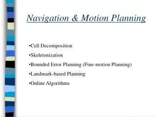
Navigation and Motion Planning for Robots. Speaker : Praveen Guddeti CSE 976, April 24, 2002. Outline. Configuration spaces. Navigation and motion planning. Cell decomposition. Skeletonization. Bounded-error planning. Landmark based navigation. Online algorithms. Conclusions.

E N D
Navigation and Motion Planning for Robots Speaker: Praveen Guddeti CSE 976, April 24, 2002
Outline • Configuration spaces. • Navigation and motion planning. • Cell decomposition. • Skeletonization. • Bounded-error planning. • Landmark based navigation. • Online algorithms. • Conclusions.
Configuration Spaces • Framework for designing and analyzing motion-planning algorithms. • Why? • State space is the all-possible configurations of the environment. • In robotics, the environment includes the body of the robot itself. • Robotics usually involves continuous state space. • Impossible to apply standard search algorithms in any straightforward way because the numbers of states and actions are infinite.
Configuration Spaces (2) • If the robot has k degrees of freedom, then the state or configuration of the robot can be described with k real values q1,…,qk. • K values can be considered as a point p in a k-dimensional space called the configuration space, C of the robot. • Set of points in C for which any part of the robot bumps into something is called the configuration space obstacle, O. • C – O is the free space, F.
Configuration Spaces (3) • Given an initial point c1 and a destination point c2 in configuration space, the robot can safely move between the corresponding points in physical space if and only if there is a continuous path between c1 and c2 that lies entirely in F. • Generalized configuration space: systems where the state of other objects is included as part of the configuration. The other objects may be movable and their shapes may vary.
Configuration Spaces (4) • E : space of all possible configurations of all possible objects in the world, other than the robot. If a given configuration can be defined by a finite set of parameters 1,…m, then E will be an m-dimensional space. • W = CE, that is W is the space of all possible configurations of the world, both robot and obstacles. • If no variation in the object shapes, then E is a single point and W and C are equivalent.
Configuration Spaces (5) • Generalized W has (k + m) degrees of freedom, but only k of these are actually controllable. • Transit paths: the paths where the robot moves freely. • Transfer paths: the paths where the robot moves an object. • Navigation in W is called a foliation. • Transit motion within any page of the book. • Transfer motion allows motion between pages.
Configuration Spaces (6) • Assumptions for planning in W: • Partition W into finitely many states. • Plan object motion first and then plan for the robot. • Restrict object motions. • Rather than a point in configuration space, if the robot starts with a probability cloud, or an envelope of possible configurations, then such an envelope is called a recognizable set.
Navigation and Motion Planning • Cell decomposition. • Skeletonization. • Bounded-error planning. • Landmark based navigation. • Online algorithms.
1. Cell Decomposition • Divide F into simple, connected regions called “cells”. This is the cell decomposition. • Determine which cells are adjacent to which others, and construct an “adjacency graph”. The vertices of this graph are cells, and edges join cells that abut each other. • Determine which cells the start and goal configurations lie in, and search for a path in the adjacency graph between those cells. • From the sequence of cells found at the last step, compute a path within each cell from a point of the boundary with the previous cell to a boundary point meeting the next cell.
Cell Decomposition (2) • Last step presupposes an easy method for navigating within cells. • F typically has complex, curved boundaries. • Two types of cell decomposition: • Approximate cell decomposition. • Exact cell decomposition.
Approximate Cell Decomposition • Approximate subdivisions using either boxes or rectangular strips. • Explicit path from start to goal is constructed by joining the midpoints of each strip with the midpoints of the boundaries with neighboring cells. • Two types of strip decomposition: • Conservative decomposition. • Reckless decomposition.
Approximate Cell Decomposition (2)Conservative Decomposition • Strips must be entirely in free space. • “Wasted” wedges of free space at the ends of strip. • What resolution of decomposition to choose? • Sound but not complete.
Approximate Cell Decomposition (3)Reckless Decomposition • Take all partially free cells as being free. • Complete but not sound.
ExactCell Decomposition • Divide free space into cells that exactly fill it. • Complex shaped cells. • Cells cylinders: • Curved top and bottom ends. • Width of cylinders not fixed. • Left and right boundaries are straight lines. • Critical points: points where the boundary curve is vertical.
2. Skeletonization • Collapse the configuration space into a one-dimensional subset, or skeleton. • Paths lie along the skeleton. • Skeleton: A web with a finite number of vertices, and paths within the skeleton can be computed using graph search methods. • Generally simpler than cell decomposition, because they provide a “minimal” description of free space.
Skeletonization (2) • To be complete for motion planning, skeletonization methods must satisfy two properties: • If S is a skeleton of free space F, then S should have a connected piece within each connected region of F. • For any point p in F, it should be “easy” to compute a path from p to the skeleton. • Skeletonization methods: • Visibility graphs. • Voronoi diagrams. • Roadmaps.
Skeletonization1. Visibility Graphs • Visibility graph for a polygonal configuration space C consists of edges joining all pairs of vertices that can see each other.
Skeletonization2. Voronoi Diagrams • For each point in free space, compute its distance to the nearest obstacle. • Plot that distance as a height coming out of the diagram. • Height of the terrain is zero at the boundary with the obstacles and increases with increasing distance from them. • Sharp ridges at points that are equidistant from two or more obstacles. • Voronoi diagrams consists of these sharp ridge points. • Complete algorithms. • Generally not the shortest path.
Skeletonization3. Roadmaps • Two curves: • Silhouette curves ( freeways). • Linking curves (bridges). • Travel on a few freeways and connecting bridges rather than an infinite space of points. • Two versions of roadways: • Silhouette method. • Extension of voronoi diagrams.
Silhouette Method • Silhouette curves are local extrema in Y of slices in X. • Linking curves join critical points to silhouette curves. Critical points are points where the cross-section X=c changes abruptly as c varies.
Extension of Voronoi Diagrams. • Silhouette curves: extremals of distance from obstacles in slices X = c. • Linking curves: start from a critical point and hill-climb in configuration space to a local maxima of the distance function.
3. Bounded-error Planning (Fine-motion Planning) • Planning small,precise motions for assembly. • Sensor and actuator uncertainly. • Plan consists of a series of guarded motions. • Motion command. • Termination condition.
Bounded-error Planning (2) • Fine-motion planner takes as input the configuration space description, the angle of velocity uncertainty cone, and a specification of what sensing is possible for termination. • Should produce a multi-step conditional plan or policy that is guaranteed to succeed, if such a plan exists. • Plans are designed for the worst case outcome. • Extremely high complexity.
4. Landmark Based Navigation • Assume the environment contains easily recognizable, unique landmarks. • A landmark is surrounded with a circular field of influence. • Robot’s control is assumed to be imperfect. • The environment is know at planning time, but not the robot’s position. • Plan backwards from the goal using backprojection. • Polynomial complexity.
5. Online Algorithms • Environment is poorly known. • Produce conditional plan. • Need to be simple. • Very fast and complete, but almost always give up any guarantee of finding the shortest path. • Competitive ratio.
Online Algorithms (2) • A complete online strategy. • Move towards the goal along the straight line L. • On encountering an obstacle stop and record the current position Q. Walk around the obstacle clockwise back to Q. Record points where the line L is crossed and the distance taken to reach them. Let P0 be the closest such point to the goal. • Walk around the obstacle from Q to P0. Now the shortest path to reach P0 is known. After reaching P0 repeat the above steps.
Conclusions • Five major classes of algorithms. • Algorithms differ in the amount of uncertainty and knowledge of the environment they require during planning time and execution time.