Download
1 / 62
690 likes | 2.06k Views
Emission and Absorption. . Chemical composition. Stellar atmosphere = mixture, composed of many chemical elements, present as atoms , ions , or molecules Abundances, e.g., given as mass fractions k Solar abundances. Universal abundance for Population I stars. Population II stars

E N D
Chemical composition • Stellar atmosphere = mixture, composed of many chemical elements, present as atoms, ions, or molecules • Abundances, e.g., given as mass fractions k • Solar abundances Universal abundance for Population I stars
Population II stars Chemically peculiar stars, e.g., helium stars Chemically peculiar stars, e.g., PG1159 stars Chemical composition
Other definitions • Particle number density Nk = number of atoms/ions of element k per unit volume • relation to mass density: • with Ak = mean mass of element k in atomic mass units (AMU) • mH = mass of hydrogen atom • Particle number fraction • logarithmic • Number of atoms per 106 Si atoms (meteorites)
Eion 6 5 4 3 2 Energy 1 The model atom • The population numbers (=occupation numbers) • ni = number density of atoms/ions of an element, which are in the level i • Ei = energy levels, quantized • E1 = E(ground state) = 0 • Eion = ionization energy free states ionization limit bound states, „levels“
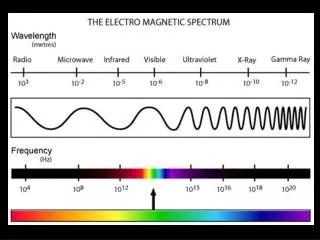
Photon absorption cross-sections • Transitions in atoms/ions • 1. bound-bound transitions = lines • 2. bound-free transitions = ionization and • recombination processes • 3. free-free transitions = Bremsstrahlung • We look for a relation between macroscopic quantities and microscopic (quantum mechanical) quantities, which describe the state transitions within an atom 3 Eion 1 2 Energie
Photon absorption cross-sections • Line transitions: • Bound-free transitions: thermal average of electron velocities v • (Maxwell distribution, i.e., electrons in thermodynamic equilibrium) • Free-free transition: free electron in Coulomb field of an ion, Bremsstrahlung, classically: jump into other hyperbolic orbit, arbitrary • For all processes holds: can only be supplied or removed by: • Inelastic collisions with other particles (mostly electrons), collisional processes • By absorption/emission of a photon, radiative processes • In addition: scattering processes = (in)elastic collisions of photons with electrons or atoms - scattering off free electrons: Thomson or Compton scattering - scattering off bound electrons: Rayleigh scattering +
The line absorption cross-section • Classical description (H.A. Lorentz) • Harmonic oscillator in electromagnetic field • Damped oscillations (1-dim), eigen-frequency 0 • Damping constant • Periodic excitation with frequency by E-field • Equation of motion: • inertia + damping + restoring force = excitation • Usual Ansatz for solution:
The line absorption cross-section • Profile function, Lorentz profile • properties: • Symmetry: • Asymptotically: • FWHM: FWHM
The damping constant • Radiation damping, classically (other damping mechanisms later) • Damping force (“friction“) • power=force velocity • electrodynamics • Hence, Ansatz for frictional force is not correct • Help: define such, that the power is correct, when time-averaged over one period: • classical radiation damping constant
Half-width • Insert into expression for FWHM:
The absorption cross-section • Definition absorption coefficient • with nlow = number density of absorbers: • absorption cross-section (definition), dimension: area • Separating off frequency dependence: • Dimension : area frequency • Now: calculate absorption cross-section of classical harmonic oscillator for plane electromagnetic wave:
Power, averaged over one period, extracted from the radiation field: • On the other hand: • Equating: • Classically: independent of particular transition • Quantum mechanically: correction factor, oscillator strength index “lu” stands for transition lower→upper level
Oscillator strengths • Oscillator strengthsflu are obtained by: • Laboratory measurements • Solar spectrum • Quantum mechanical computations (Opacity Project etc.) • Allowed lines: flu1, • Forbidden: <<1 e.g. He I 1s2 1S1s2s 3S flu=210-14
Opacity status report • Connecting the (macroscopic) opacity with (microscopic) atomic physics • View atoms as harmonic oscillator • Eigenfrequency: transition energy • Profile function: reaction of an oscillator to extrenal driving (EM wave) • Classical crossection: radiated power = damping Classical crossection Profile function QM correction factor Population number of lower level
Extension to emission coefficient • Alternative formulation by defining Einstein coefficients: • Similar definition for emission processes: • profile function, complete redistribution:
Relations between Einstein coefficients • Derivation in TE; since they are atomic constants, these relations are valid independent of thermodynamic state • In TE, each process is in equilibrium with its inverse, i.e., within one line there is no netto destruction or creation of photons (detailed balance)
Relation to oscillator strength • dimension • Interpretation of as lifetime of the excited state • order of magnitude: • at 5000 Å: • lifetime:
Comparison induced/spontaneous emission • When is spontaneous or induced emission stronger? • At wavelengths shorter than spontaneous emission is dominant
Induced emission as negative absorption • Radiation transfer equation: • Useful definition: corrected for induced emission: transition low→up So we get (formulated with oscillator strength instead of Einstein coefficients):
The line source function • General source function: • Special case: emission and absorption by one line transition: • Not dependent on frequency • Only a function of population numbers • In LTE:
Line broadening: Radiation damping • Every energy level has a finite lifetime against radiative decay (except ground level) • Heisenberg uncertainty principle: • Energy level not infinitely sharp • q.m. profile function = Lorentz profile • Simple case: resonance lines (transitions to ground state) • example Ly (transition 21): • example H (32):
Line broadening: Pressure broadening • Reason: collision of radiating atom with other particles • Phase changes, disturbed oscillation t0 = time between two collisions
Line broadening: Pressure broadening • Semi-classical theory (Weisskopf, Lindholm), „Impact Theory“ • Phase shifts : • find constants Cpby laboratory measurements, or calculate • Good results for p=2 (H, He II): „Unified Theory“ • H Vidal, Cooper, Smith 1973 • He II Schöning, Butler 1989 • For p=4 (He I) • Barnard, Cooper, Shamey; Barnard, Cooper, Smith; Beauchamp et al. Film logg
Thermal broadening • Thermal motion of atoms (Doppler effect) • Velocities distributed according to Maxwell, i.e. • for one spatial direction x (line-of-sight) • Thermal (most probable) velocity vth:
Line profile • Doppler effect: • profile function: • Line profile = Gauss curve • Symmetric about 0 • Maximum: • Half width: • Temperature dependency: FWHM
Examples • At 0=5000Å: • T=6000K, A=56 (Fe): th=0.02Å • T=50000K, A=1 (H): th=0.5Å • Compare with radiation damping: FWHM=1.18 10-4Å • But: decline of Gauss profile in wings is much steeper than for Lorentz profile: • In the line wings the Lorentz profile is dominant
Line broadening: Microturbulence • Reason: chaotic motion (turbulent flows) with length scales smaller than photon mean free path • Phenomenological description: • Velocity distribution: • i.e., in analogy to thermal broadening • vmicrois a free parameter, to be determined empirically • Solar photosphere: vmicro =1.3 km/s
Joint effect of different broadening mechanisms • Mathematically: convolution • commutative: • multiplication of areas: • Fourier transformation: y x y x profile A + profile B = joint effect x i.e.: in Fourier space the convolution is a multiplication
Application to profile functions • Convolution of two Gauss profiles (thermal broadening + microturbulence) • Result: Gauss profile with quadratic summation of half-widths; proof by Fourier transformation, multiplication, and back-transformation • Convolution of two Lorentz profiles (radiation + collisional damping) • Result: Lorentz profile with sum of half-widths; proof as above
Application to profile functions • Convolving Gauss and Lorentz profile (thermal broadening + damping)
Treatment of very large number of lines • Example: bound-bound opacity for 50Å interval in the UV: • Direct computation would require very much frequency points • Opacity Sampling • Opacity Distribution Functions ODF (Kurucz 1979) Möller Diploma thesis Kiel University 1990
Bound-free absorption and emission • Einstein-Milne relations, Milne 1924: Generalization of Einstein relations to continuum processes: photoionization and recombination • Recombination spontaneous + induced • Transition probabilities: • I) number of photoionizations • II) number of recombinations • Photon energy • In TE, detailed balancing: I) = II)
Einstein-Milne relations • Einstein-Milne relations, continuum analogs to Aji, Bji, Bij
Absorption and emission coefficients definition. of cross-section • absorption coefficient (opacity) • emission coefficient (emissivity) • And again: induced emission as negative absorption • and (using Einstein-Milne relations) • LTE:
Continuum absorption cross-sections • H-like ions: semi-classical Kramers formula • Quantum mechanical calculations yield correction factors • Adding up of bound-free absorptions from all atomic levels: example hydrogen
Continuum absorption cross-sections Optical continuum dominated by Paschen continuum
The solar continuum spectrum and the H- ion • H- ion has one bound state, ionization energy 0.75 eV • Absorption edge near 17000Å, • hence, can potentially contribute to opacity in optical band • H almost exclusively neutral, but in the optical Paschen-continuum, i.e. population of H(n=3) decisive: • Bound-free cross-sections for H- and H0 are of similar order • H- bound-free opacity therefore dominates the visual continuum spectrum of the Sun
The solar continuum spectrum and the H- ion Ionized metals deliver free electrons to build H-
Free-free absorption and emission • Assumption (also valid in non-LTE case): • Electron velocity distribution in TE, i.e. Maxwell distribution • Free-free processes always in TE • Similar to bound-free process we get: • generalized Kramers formula, with Gauntfaktor from q.m. • Free-free opacity important at higher energies, because less and less bound-free processes present • Free-free opacity important at high temperatures
Computation of population numbers • General case, non-LTE: • In LTE, just • In LTE completely given by: • Boltzmann equation (excitation within an ion) • Saha equation (ionization)
Boltzmann equation • Derivation in textbooks • Other formulations: • Related to ground state (E1=0) • Related to total number density N of respective ion
Divergence of partition function • e.g. hydrogen: • Normalization can be reached only if number of levels is finite. • Very highly excited levels cannot exist because of interaction with neighbouring particles, radius H atom: • At density 1015 atoms/cm3 mean distance about 10-5 cm • r(nmax) = 10-5 cm nmax ~43 • Levels are “dissolved“; description by concept of occupation probabilities pi (Mihalas, Hummer, Däppen 1991)