Download
1 / 98
980 likes | 1.14k Views
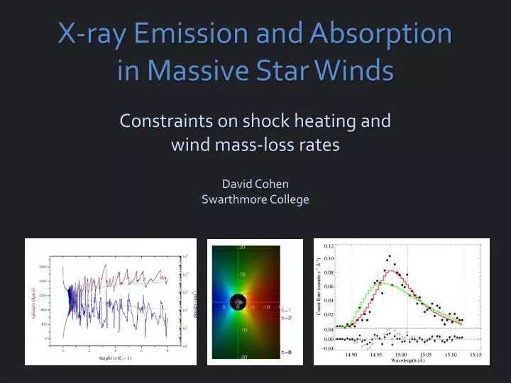
X-ray Emission and Absorption in Massive Star Winds. David Cohen Swarthmore College. Constraints on shock heating and wind mass-loss rates. What we know about X-rays from single O stars. David Cohen Swarthmore College. via high-resolution spectroscopy. Outline. Morphology of X-ray spectra

E N D
X-ray Emission and Absorption in Massive Star Winds David CohenSwarthmore College Constraints on shock heating and wind mass-loss rates
What we know about X-rays from single O stars David CohenSwarthmore College via high-resolution spectroscopy
Outline • Morphology of X-ray spectra • Embedded Wind Shocks: X-ray diagnostics of kinematics and spatial distribution • Line profiles and mass-loss rates • Broadband absorption
Morphology Pup (O4 If) Capella(G5 III) – coronal source – for comparison
Si XIV Mg XII Ne X Fe XVII Ne IX Si XIII Mg XI Pup (O4 If) Capella(G5 III) – coronal source – for comparison
H-like vs. He-like Si XIV Mg XII Ne X Ne IX Si XIII Mg XI Pup (O4 If) Capella(G5 III) – coronal source – for comparison
H-like vs. He-like Mg XII Mg XI Pup (O4 If) Capella(G5 III) – coronal source – for comparison
H-like vs. He-like Mg XII Mg XI Pup (O4 If) Capella(G5 III) – coronal source – for comparison
Spectral energy distribution trends • The O star has a harder spectrum, but apparently cooler plasma We’ll see later on that soft X-ray absorption by the winds of O stars explains this
Next • First, we’ll look at what can be learned about the kinematics and location of the X-ray emitting plasma from the emission lines • After that, we’ll look at the issues of wind absorption and its effects on line shapes and on the broadband hardness trend
Embedded wind shocks • Numerical simulations of the line-driven instability (LDI) predict: • Distribution of shock-heated plasma • Above an onset radius of r~ 1.5 R*
1-D rad-hydro simulations • Self-excited instability (smooth initial conditions)
Vshock ~ 300 km/s : T ~ 106 K shock onset at r ~ 1.5 Rstar pre-shock wind plasma has low density
Vshock ~ 300 km/s : T ~ 106 K shock onset at r ~ 1.5 Rstar Shocked wind plasma is decelerated back down to the local CAK wind velocity
Morphology Pup (O4 If) Capella(G5 III) – coronal source – for comparison
Ne IX Fe XVII Ne X Morphology – line widths Pup (O4 If) Capella(G5 III) – coronal source – for comparison
Ne IX Fe XVII Ne X Morphology – line widths Pup (O4 If) ~2000 km/s ~ vinf Capella(G5 III) – coronal source – for comparison
Shock heated wind plasma is moving at >1000 km/s : broad X-ray emission lines
99% of the wind mass is cold*, partially ionized…x-ray absorbing opacity *typically 20,000 – 30,000 K; maybe better described as “warm”
x-ray absorption is due to bound-free opacity of metals opacity …and it takes place in the 99% of the wind that is unshocked
Emission + absorption = profile model • The kinematics of the emitting material dictates the line width and overall profile • Absorption affects line shapes
Onset radius of X-ray emission, Ro isovelocity contours -0.2vinf +0.2vinf -0.6vinf +0.6vinf -0.8vinf +0.8vinf observer on left
isovelocity contours -0.2vinf +0.2vinf -0.6vinf +0.6vinf -0.8vinf +0.8vinf observer on left t= 3 optical depth contours t= 1 t= 0.3
Profile shape assumes beta velocity law and onset radius, Ro
Universal property of the wind zdifferent for each point
opacity of the cold wind wind mass-loss rate wind terminal velocity radius of the star
= 1 contours t=1,2,8 Ro=1.5 Ro=3 j ~ 2 for r/R* > Ro = 0 otherwise Ro=10 key parameters: Ro &t*
We fit these x-ray line profile models to each line in the Chandra data Fe XVII Fe XVII
And find a best-fit t* and Ro… t* = 2.0 Ro = 1.5 Fe XVII Fe XVII
…and place confidence limits on these fitted parameter values 68, 90, 95% confidence limits
Let’s focus on the Ro parameter first Note that for b = 1, v = 1/3 vinf at 1.5 R* and 1/2 vinf at 2 R*
Wind Absorption CNO processed • Next, we see how absorption in the bulk, cool, partially ionized wind component affects the observed X-rays Solar opacity
Morphology Pup (O4 If) Capella(G5 III) – coronal source – for comparison
Ne IX Fe XVII Ne X Morphology – line widths Pup (O4 If) ~2000 km/s ~ vinf Capella(G5 III) – coronal source – for comparison
Pup (O4 If) Capella(G5 III) – unresolved
opacity of the cold wind wind mass-loss rate t*is the key parameter describing the absorption wind terminal velocity radius of the star
t* = 2 in this wind -0.2vinf +0.2vinf -0.6vinf +0.6vinf -0.8vinf +0.8vinf observer on left t= 3 optical depth contours t= 1 t= 0.3
Wind opacity • X-ray bandpass
Wind opacity • X-ray bandpass Chandra HETGS
X-ray opacity CNO processed • Zoom in Solar
We fit these x-ray line profile models to each line in the Chandra data Fe XVII Fe XVII