Download
1 / 24
240 likes | 410 Views
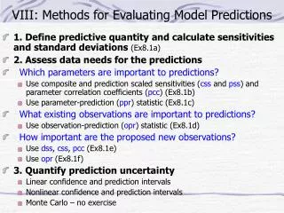
VIII: Methods for Evaluating Model Predictions. 1. Define predictive quantity and calculate sensitivities and standard deviations (Ex8.1a) 2. Assess data needs for the predictions Which parameters are important to predictions?

E N D
VIII: Methods for Evaluating Model Predictions • 1. Define predictive quantity and calculate sensitivities and standard deviations (Ex8.1a) • 2. Assess data needs for the predictions • Which parameters are important to predictions? • Use composite and prediction scaled sensitivities (css and pss) and parameter correlation coefficients (pcc) (Ex8.1b) • Use parameter-prediction (ppr) statistic (Ex8.1c) • What existing observations are important to predictions? • Use observation-prediction (opr) statistic (Ex8.1d) • How important are the proposed new observations? • Use dss, css, pcc (Ex8.1e) • Use opr (Ex8.1f) • 3. Quantify prediction uncertainty • Linear confidence and prediction intervals • Nonlinear confidence and prediction intervals • Monte Carlo – no exercise
Exercise files • MFI2005 does not support predictions • All the files have been constructed for you, and are in initial\ex8.i • Copy the files to exer\ex8 • Execute batch files as described in the input instructions. • Look at output files • For other problems, you can use the class files as a beginning point.
Define predictive quantity • We typically make predictions to assess the state of the simulated system at a future time. • Often, predictions occur under different conditions than those under which the model was calibrated – addition of pumping, change in boundary conditions, etc. • The predictive quantity might differ from the types of quantities used as observations. • You as the modeler need to help define what model-calculated values are best to use as predictions in the problem of concern • The predictions available can depend on the software used • MODFLOW-2005: any quantity that can be an observation can also be a prediction. Heads, temporal changes in head, some flows, advective transport. • UCODE_2005 or PEST: any quantity that can be calculated using values in the application model output files.
Prediction sensitivities (Book, p. 159) • Used to calculate measures for assessing: • Parameters important to predictions • Observations important to predictions • Prediction uncertainty • Data needs • Prediction sensitivities: • Usually need to scale these sensitivities to produce useful measures.
Prediction scaled sensitivities (pss)(Book, p. 160-161) • Scaling depends on prediction and purpose. Four useful scalings are: 1.pss is percent change in prediction caused by a 1-percent change in the parameter value bj (in _sppp file of UCODE_2005): pssj = (zl/ bj) (bj/100) (100/zl) 2. pss is percent change in prediction caused by a change in bj equal to 1 percent of its standard deviation sbj(in _spsp file): pssj = (zl/ bj) (sbj/100) (100/zl) 3,4. For both these scalings, (100/zl) can be replaced by (100/al), where a’ is some other meaningful quantity. On p. 161, using a reference value is suggested. (in _sppr and _spsr file of UCODE_2005) In _sp** , third letter identifies parameter value or standard deviation on the parameter; fourth letter identifies prediction or reference value)
Parameter Correlation Coefficients (pcc) in the Context of Predictions (Book, p. 162-166) • Calculate pcc using different combinations of observations, prior, and predictions to evaluate the existence and need for unique parameter estimates • For example, two parameters are extremely correlated given a set of observations. This is only a problem if the predictions need unique values. • Next: Use pss, css, and pcc together to assess the importance of parameters to the predictions.
Use pss and css to identify insensitivity problems Are imprecise parameter estimates important to the predictions? (from Hill & Tiedeman, Figure 8.2a, p. 166)
Use pcc to identify uniqueness problems Are non-unique parameter estimates important to the predictions? (from Hill & Tiedeman, Figure 8.2b, p. 166)
Prediction Exercises – Book, p. 193-212 • Developer claims landfill effluent will go to river, not to wells. • Water supply wells are being completed and a pump test could be used to collect more data on the system. • Developer claims the model is inadequate for two reasons: • Model was calibrated using heads and flows and no pumping, but is being used to predict advective transport under pumping conditions. • Need for prior suggests the observations are inadequate • County government officials want to know: • Is existing model adequate? • Wait for new data? • We, as the modelers, suggest using sensitivity analysis to: • Evaluate the developer’s claims. • Plan new data collection
Predicted transport from landfill ? ? Will effluent go to well or river? Thorough analysis requires full transport model (advection, dispersion, etc.). We will do preliminary analysis using Advective Transport. Use MODPATH.
Predictions simulated using MODPATH(Pollock 1996) • Calculates motion in the x, y and z directions. • When used for observations: • Observed advective transport inferred from concentrations. • Three entries are added to the objective function for each advective-transport observation. • When used for predictions: • Three predictions for each advective transport prediction – transport along rows (y), columns (x), and vertically (z). • Calculates sensitivities; these are used here to calculate pcc, parameter standard deviations, and linear confidence intervals.
Particle path simulated using MODPATH. The horizontal and vertical bars show one standard deviation at selected travel times. Start of path End of path
Predictive transport: Questions to address (p. 194) • Transport destination and time? Ex. 8.1a. • Forward model with MODPATH • Consider the parameters important to predictions. Are they precisely and uniquely estimated? • Prediction and composite scaled sensitivities and parameter correlation coefficients (pss, css, pcc). Ex. 8.1b. • PPR statistic. Ex. 8.1c • What existing observations are important? • OPR statistic. Ex. 8.1d • Are potential new observations worth waiting for? • Dimensionless and prediction scaled sensitivities, parameter correlation coefficients (dss, pss, pcc). Ex. 8.1e • OPR statistic. Ex. 8.1f • What is the prediction uncertainty? • Linear confidence intervals. Ex. 8.2a. • Nonlinear confidence intervals. Ex 8.2b.
Exercise 8.1a: Predict Advective Transport Read general Exercises description on p. 193-195. Do Exercise 8.1a on p. 195-196 In the simulation, where does the landfill effluent go, and how long does it take to get there?
@ [ MODPATH Version 4.00 (V4, Release 3, 7-2003) (TREF= 0.000000E+00 ) ] 1 1.55000E+04 1.65000E+04 9.99900E-01 9.99950E+01 0.00000E+00 16 2 1 1 1 1.51565E+04 1.63903E+04 7.87957E-01 8.93978E+01 -3.15000E+08 16 2 1 1 1 1.51565E+04 1.63903E+04 7.87957E-01 8.93978E+01 3.15000E+08 16 2 1 1 1 1.50000E+04 1.63422E+04 7.10433E-01 8.55216E+01 4.46763E+08 15 2 1 1 1 1.40917E+04 1.60000E+04 4.02401E-01 7.01200E+01 1.11285E+09 15 3 1 1 1 1.40000E+04 1.59693E+04 3.82440E-01 6.91220E+01 1.16709E+09 14 3 1 1 1 1.32700E+04 1.56553E+04 2.56172E-01 6.28086E+01 -1.57000E+09 14 3 1 1 1 1.32700E+04 1.56553E+04 2.56172E-01 6.28086E+01 1.57000E+09 14 3 1 1 1 1.30000E+04 1.55379E+04 2.19734E-01 6.09867E+01 1.70786E+09 13 3 1 1 1 1.20897E+04 1.50000E+04 1.26071E-01 5.63035E+01 2.14586E+09 13 4 1 1 1 1.20000E+04 1.49508E+04 1.19582E-01 5.59791E+01 2.18187E+09 12 4 1 1 1 1.10000E+04 1.41688E+04 5.97149E-02 5.29857E+01 2.58234E+09 11 4 1 1 1 1.08476E+04 1.40000E+04 5.20098E-02 5.26005E+01 2.64385E+09 11 5 1 1 1 1.00382E+04 1.30000E+04 1.70220E-02 5.08511E+01 2.94240E+09 11 6 1 1 1 1.00000E+04 1.29501E+04 1.52036E-02 5.07602E+01 2.95493E+09 10 6 1 1 1 9.76378E+03 1.25238E+04 0.00000E+00 5.00000E+01 3.03896E+09 10 6 1 1 1 9.76378E+03 1.25238E+04 -3.23767E-01 4.67623E+01 -3.15000E+09 10 6 1 1 1 9.76378E+03 1.25238E+04 -3.23767E-01 4.67623E+01 3.15000E+09 10 6 1 1 1 9.76378E+03 1.25238E+04 1.00000E+00 4.00000E+01 3.38193E+09 10 6 2 1 1 9.56571E+03 1.20000E+04 9.22715E-01 3.61357E+01 3.83712E+09 10 7 2 1 1 9.38455E+03 1.10000E+04 6.69144E-01 2.34572E+01 4.32990E+09 10 8 2 1 1 9.38417E+03 1.00000E+04 3.71525E-01 8.57624E+00 4.49415E+09 10 9 2 1 MODPATH Output (Equivalent to ADV output on Fig. 8.7a, p. 196 Level above bottom of model layer Distance along columns from bottom Time, in seconds Level above bottom of model Distance along rows from left Row, column, layer
Exercise 8.1b: Determine problematic parameters using css and pss • Compare prediction and composite scaled sensitivities: Are pss large for any parameters with small css? • Use pss scaling so that pss represent the percent change in distance traveled caused by a 1-percent change in a parameter value: pssj = (zl/ bj) (bj/100) |100/zl| One-percent scaled sens For UCODE_2005, these pss are in ex8.1b \ ex8.1b_sppp.
Exercise 8.1b: Determine problematic parameters using pcc • Compare two different sets of parameter correlation coefficients: • pcc calculated using only calibration observations • pcc calculated with calibration observations AND predictions. • Use parameter correlation coeffeicients in ex8.1b \ ex8.1b._mc or _pcc • ex8.1b-obs-pred\
Exercise 8.1b: Prediction weights needed forpcc with predictions • Weights for the advective travel predictions are calculated from specified standard deviations, in meters (Table 8.3, p. 198). • Weights in this analysis can reflect desired prediction precision. • Do Exercise 8.1b (p. 196-199) and the Problems. • Question 2: Are parameters important to predictions precisely and uniquely estimated?
Results of Exercise 8.1bcss-pss analysis for Question 2: Are parameters important to predictions preciselyestimated? Figure 8.8, p. 198
Results of Exercise 8.1bcss-pss analysis for Question 2: Are parameters important to predictions preciselyestimated? Not all of them Figure 8.8, p. 198
Results of Exercise 8.1b pcc analysis for Question 2: Are parameters important to predictions uniquelyestimated? Observations only Not all of them No correlations larger than 0.85 Tables 8.4 & 8.5, p. 199 With predictions
Exercise 8.1c: PPR Individual Parameters Average ppr statistic for all predictions Figure 8.9a, p. 201 Which parameters rank as most important to the predictions by the ppr statistic? How does this differ from the rankings by the pss? What causes these differences?
Response to developer concerns • Developer claims the model is inadequate for two reasons: • Model was calibrated using heads and flows and no pumping, but is being used to predict advective transport under pumping conditions. • Need for prior suggests the observations are inadequate • Our response based on sensitivity analysis • Indeed, the model is inadequate. • The calibration data does not provide information on some parameters important to predictions • Also, we stress that we need to consider the results of an uncertainty analysis