Download
1 / 58
600 likes | 755 Views
Functional Mapping of QTL and Recent Developments. Chang-Xing Ma Department of Biostatistics University at Buffalo cxma@buffalo.edu Rongling Wu University of Florida. Outline. Interval Mapping Functional Mapping Functional Mapping Demo Recent Developments Conclusion.

E N D
Functional Mapping of QTLand Recent Developments Chang-Xing Ma Department of Biostatistics University at Buffalo cxma@buffalo.edu Rongling Wu University of Florida
Outline • Interval Mapping • Functional Mapping • Functional Mapping Demo • Recent Developments • Conclusion
Gene, Allele, Genotype, Phenotype Chromosomes from FatherMother Genotype Phenotype Height IQ AA 185 100 AA 182 104 Gene A, with two alleles A and a Aa 175 103 Aa 171 102 aa 155 101 aa 152 103
Regression model for estimating the genotypic effect Phenotype = Genotype + Error yi = xij + ei xiis the indicator for QTL genotype jis the mean for genotype j ei ~ N(0, 2)
The genotypes for the trait are not observable and should be predicted from linked neutral molecular markers (M) M1 QTL M2 The genes that lead to the phenotypic variation are called Quantitative Trait Loci (QTL) M3 . . . Our task is to construct a statistical model that connects the QTL genotypes and marker genotypes through observed phenotypes Mm
Data Structure Parents AA aa F1Aa F2AA Aa aa ¼ ½ ¼ n = n22 + n21 + n20 + n12 + n00 + n02 + n01 + n00
Finite mixture model for estimating genotypic effects yi ~ p(yi|,) = ¼ f2(yi) + ½ f1(yi) + ¼ f0(yi) QTL genotype (j) QQQqqq Code 210 where fj(yi) is a normal distribution density with mean jand variance 2 = (2, 1, 0), = (2)
L(, , |M, y) Likelihood function based on the mixture model j|i is the conditional (prior) probability of QTL genotype j (= 2, 1, 0) given marker genotypes for subject i (= 1, …, n).
We model the parameters contained within the mixture model using particular functions QTL genotype frequency: j|i = gj(p) Mean: j= hj(m) Variance: = l(v) • p contains the population genetic parameters • q = (m, v) contains the quantitative genetic parameters
r=a+b-2ab j|i F2QTL genotype frequency: M a Q b N 2|22 1|12
Log- Likelihood Function
The EM algorithm E step Calculate the posterior probability of QTL genotype j for individual i that carries a known marker genotype M step Solve the log-likelihood equations Iterations are made between the E and M steps until convergence
Interval Mapping Program - Type of Study - Genetic Design
Interval Mapping Program - Data and Options Names of Markers (optional) Cumulative Marker Distance (cM) Map Function QTL Searching Step cM Parameters Here for Simulation Study Only
Interval Mapping Program - Data Put Markers and Trait Data into box below OR
Interval Mapping Program - Analyze Data Trait:
Interval Mapping Program - Profile
Interval Mapping Program - Permutation Test #Tests Cut off Point at Level Is Based on Tests.
Functional Mapping An innovative model for genetic dissection of complex traits by incorporating mathematical aspects of biological principles into a mapping framework Provides a tool for cutting-edge research at the interplay between gene action and development
Parents AA aa F1Aa F2AAAa aa ¼ ½ ¼ Data Structure n = n22 + n21 + n20 + n12 + n00 + n02 + n01 + n00
The Finite Mixture Model Observation vector,yi = [yi(1), …, yi(T)] ~ MVN(uj, ) Mean vector, uj = [uj(1), uj(2), …, uj(T)], (Co)variance matrix,
Modeling the Mean Vector • Parametric approach Growth trajectories – Logistic curve HIV dynamics – Bi-exponential function Biological clock – Van Der Pol equation Drug response – Emax model • Nonparametric approach Lengedre function (orthogonal polynomial) B-spline
Stem diameter growth in poplar trees Ma, Casella & Wu: Genetics 2002
Logistic Curve of Growth – A Universal Biological Law (West et al.: Nature 2001) Logistic Curve of Growth – A Universal Biological Law Instead of estimating uj, we estimate curve parameters q= (aj, bj, rj) Modeling the genotype- dependent mean vector, uj = [uj(1), uj(2), …, uj(T)] = [ , , …, ] Number of parameters to be estimated in the mean vector Time points Traditional approach Our approach 5 3 5 = 15 3 3 = 9 10 3 10 = 30 3 3 = 9 50 3 50 = 150 3 3 = 9
Modeling the Variance Matrix Stationary parametric approach Autoregressive (AR) model Nonstationary parameteric approach Structured antedependence (SAD) model Ornstein-Uhlenbeck (OU) process Nonparametric approach Lengendre function
Autoregressive model AR(1) = q= (aj, bj, rj , ρ, σ2)
Box-Cox Transformation Differences in growth across ages Untransformed Log-transformed Poplar data
EM Algorithm (Ma et al 2002, Genetics) Estimate (aj, bj, rj; rho, sigma^2)
An example of a forest tree The study material used was derived from the triple hybridization of Populus (poplar). A Populus deltoides clone (designated I-69) was used as a female parent to mate with an interspecific P. deltoides x P. nigra clone (designated I-45) as a male parent (WU et al. 1992 ). In the spring of 1988, a total of 450 1-year-old rooted three-way hybrid seedlings were planted at a spacing of 4 x 5 m at a forest farm near Xuchou City, Jiangsu Province, China. The total stem heights and diameters measured at the end of each of 11 growing seasons are used in this example. A genetic linkage map has been constructed using 90 genotypes randomly selected from the 450 hybrids with random amplified polymorphic DNAs (RAPDs) (Yin 2002)
Functional mapping incorporated by logistic curves and AR(1) model QTL
Functional Mapping - Data Genetic Design: Curve: Marker Place: Time Point: Parameters Here for Simulation Study QTL Position: Sample Size: Curve Parameters: Sigma^2: Correlation rho: cM Map Function: Search Step:
Functional Mapping - Data Put Markers and Trait Data into box below OR
Functional Mapping - Data Curves
Functional Mapping - Profile Initiate Values
Functional Mapping - Profile
Functional Mapping - Data Curves
Recent Developments • transform-both-sides logistic model. Wu, Ma, et al Biometrics 2004 • Multiple genes – Epistatic gene-gene interactions. Wu, Ma, et al Genetics 2004 • Multiple environments – Genotype x environment Zhao,Zhu,Gallo-Meagher & Wu: Genetics 2004 • Multiple traits – Trait correlationsZhao et al Biometrics 2005 • Genetype by Sex interactions - Zhao,Ma,Cheverud &Wu Physiological Genomics 2004
transform-both-sides logistic model Developmental pattern of genetic effects Wu, Ma, Lin, Wang & Casella: Biometrics 2004 Timing at which the QTL is switched on
Functional mapping for epistasis in poplar Wu, Ma, Lin & Casella Genetics 2004 QTL 1 QTL 2
Functional mapping for epistasis in poplar The growth curves of four different QTL genotypes for two QTL detected on the same linkage group D16
Genotype environment interaction in rice Zhao, Zhu, Gallo-Meagher & Wu: Genetics 2004
Plant height growth trajectories in rice affected by QTL in two contrasting environments Red: Subtropical Hangzhou Blue: Tropical Hainan QQ qq
Functional mapping: Genotype sex interaction Zhao, Ma, Cheverud & Wu Physiological Genomics 2004
Body weight growth trajectories affected by QTL in male and female mice QQ Qq qq Red: Male mice Blue: Female mice
Functional mapping for trait correlation Zhao, Hou, Littell & Wu: Biometrics submitted
Growth trajectories for stem height and diameter affected by a pleiotropic QTL Red: Diameter Blue: Height QQ Qq
Functional Mapping:toward high-dimensional biology • A new conceptual model for genetic mapping of complex traits • A systems approach for studying sophisticated biological problems • A framework for testing biological hypotheses at the interplay among genetics, development, physiology and biomedicine
Functional Mapping:Simplicity from complexity • Estimating fewer biologically meaningful parameters that model the mean vector, • Modeling the structure of the variance matrix by developing powerful statistical methods, leading to few parameters to be estimated, • The reduction of dimension increases the power and precision of parameter estimation