Download
1 / 28
280 likes | 541 Views
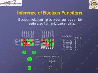
Inference of Boolean Functions. Boolean relationship between genes can be estimated from microarray data. Experiment 1. Experiment 2. Experiment 3. Experiment 4. Experiment 5. Experiment 6. Experiment 1. Experiment 2. Experiment 3. Experiment 4. Experiment 5. Experiment 6. Examples:

E N D
Inference of Boolean Functions Boolean relationship between genes can be estimated from microarray data. Experiment 1 Experiment 2 Experiment 3 Experiment 4 Experiment 5 Experiment 6 Experiment 1 Experiment 2 Experiment 3 Experiment 4 Experiment 5 Experiment 6 Examples: A B C Experiment 1 0 0 1 Experiment 2 0 1 0 Experiment 3 1 1 0 Experiment 4 1 1 1 Experiment 5 1 1 1 Experiment 6 0 0 1 Gene A Gene A 0 0 1 1 1 0 Gene B Gene B 0 1 1 1 1 0 Gene C Gene C 1 0 0 1 1 1 Gene D Gene D 1 0 0 0 1 1 A B Boolean function fc for C A B C 0 0 1 0 1 0 1 0 X 1 1 1 fC C
Connectivity of BN • Predictor set for BN: W := (W1,…, Wn) • Minimum predictor set ~ BN Connectivity • Compatibility between W and the state transition diagram • BN Connectivity and its relation to the regime of functioning: ordered, chaotic or on the edge of chaos
State Transition Diagram 100 000 101 110 111 001 010 011
Interpretation of the State Transition Diagrams • Attractors/fixed points ~ cellular types or cellular states, such as proliferation, apoptosis, and differentiation • Basins of attraction ~ structural stability or ordered collective behavior * Stuart A. Kaufman, Origin of Order : ‘Self-Organization and Selection in Evolution’, Oxford Univ. Press, 1993
Problem: to find the connection between genes Gene 4 Gene 2 Gene 3 Gene 5 Gene 1 Gene space CoD Gene 1 Gene 2 Gene 3 Gene 4 Gene 5 Gene 1 Gene 2 Gene 3 Gene 4 Gene 5
Error measure for binary functions • How good is this function to “model” the relationship between G1,G2 and G3 ? • The quality of the function depends on the “joint” distribution of G1,G2 and G3 • In the same way, if the constant function is defined by 0=c
G1 G2 G3 Boolean Functions • If the expression of the genes is assumed to have 2 possible values (0 – inactive,1 - active), we can use Boolean functions to “model” the relationship between the genes. One example of a Boolean function All possible combination of values for the pair {G1,G2}
G1 G2 G3 Constant Functions • The behavior of the gene G3 can also be predicted by a constant function. • In this case G3 doesn’t depend on G1 and G2, so we can write “ = 0 = c ” to specify the function (The sub-index 0 in 0 denotes the absence of predictors) Example of a constant function
Optimal Function • Between all possible Boolean functions , one of them has the minimal error, as predictor of G3 from G1 and G2. This function is called opt. • [opt] [] for any other Boolean function • If G1 and G2 are good predictors of G3, then the relationship between them will be “captured” by optand [opt] will be small. • The optimal constant predictor is called 0-opt. (there are only 2 possible constant predictors: 0 and 1). • If G3 is almost constant, then [0-opt] will be small.
Coefficient of Determination • The Coefficient of Determination (CoD) of the pair of genes G1 and G2 as predictors of the gene G3 is given by the relative improvement in the prediction when using the optimal predictor optover the optimal constant predictor 0-opt. • The CoD depends ONLY on the joint distribution of G1,G2 and G3.
Estimation of the CoD for G1,G2 and G3. Microarrays Example of a Binary Expression Matrix Estimation of the optimal functions optand 0-optfor {G1,G2} as predictors of G3 Estimated CoD for {G1,G2} as predictors of G3
Estimation of [opt] for G1,G2 and G3 from the data Ternary Expression Matrix for G1,G2 and G3 Splitting of the matrix in Training and Test sets
Estimation of [opt] for G1,G2 and G3 from the data More frequent value computed from data (X denotes a non- observed configuration) Generalization to fill non-observed configurations Statistical Inference of the optimal function opt. Estimation of the error of [opt] from test set 1 mistake on 4 *[opt]= 0.25
Estimation of [0-opt] for G1,G2 and G3 from the data Frequencies of possible values of G3 on train data Statistical Inference of the optimal function 0-opt. 0-opt. = 1(use heuristic) (most frequently observed value for G3) Estimation of the error of [opt] from test set 3 mistakes on 4 *[0-opt]= 0.75
Estimation of the CoD for G1,G2 and G3 from the data *[opt]= 0.25 *[0-opt]= 0.75 The error is reduced in a 66 %
Estimation of the CoD for G1,G2 and G3. • The previous process is repeated 1000 times, with different random splitting of the set in training and test sets. • The estimated value for the CoD is the average of the 1000 values of *. • If we want to know the predictive power of other pair of genes, say G4,G5, over G3, we must repeat the whole process • G1,G2 G3 312 • G4,G5 G3 345
Methodology • Compute the CoD for all sets of 1,2 and 3 predictors for each target gene. 1 predictor 2 predictors 3 predictors Gene 2 Gene 2 & 3 Gene 3 & 4 Gene 2,3,4 Gene 3 Gene 2 & 4 Gene 3 & 5 Gene 2,3,5 Gene 4 Gene 2 & 5 Gene 4 & 5 Gene 2,4,5 Gene 5 Gene 3,4,5 Gene 1 Quality of prediction : CoD
Results • Most probable predictors sets for each gene Gene 2 Gene 2, 3 Gene 2,3,4 Gene 1 2 23 234
Gene 1 Gene 2 Gene 3 Gene 4 Gene 5 Gene 1 Gene 2 Gene 3 Gene 4 Gene 5 Results • Determination of the predictive genetic network
Discussion • The CoD can be applied to ternary data, more general discrete data and on continuous data, restricting the family of functions (linear, neural network, etc) • This technique is a “feature selection” technique analyzing all the possibilities. Existing algorithms can be applied to optimize the search, in detriment of the quality of the result (ex: genetic algorithm, sub-optimal search)
Conclusions about CoD • CoD is a useful tool in the determination of the predictive genetic network • Computationally expensive: feasible only for 3 predictor sets for moderate sets 200-500 genes • Does not give information about the functions, but they can be estimated easily from the data
Regulatory diagram for the activation of the tumor-suppressor protein p53 Vogelstein, B., Lane, D. &Levine, A. Surfing the p53 network. Nature 408, 307-310 (2000)
Formulate the question Organizing and cleaning data Interpretation of results Normalize data Analyze data
The question(s) • Team 1: What are the differences of gene profiles between fish oil group and corn oil group in AOM injected rats? (same for the olive and the corn oil groups) • Team 2: Find DE, with respect to treatment (AOM vs. Saline), genes. • Team 3: Find DE, with respect to the 2 time points, genes for the AOM treated animals. Same question for the saline treated animals. • Team 4: Find DE, with respect to the treatment type, genes for the animals sacrificed at the first time point. Same for the second time point.
Presentations 27.07.09 (1 presentation: Team 1) 28.07.09 (2 presentations: Team 3, Team 2) 29.07.09 (1 presentation: Team 4)
Quiz #2 Everything from Quiz #1 up to and including Lecture #6