Microarray Data Analysis
Microarray Data Analysis. The Bioinformatics side of the bench. The anatomy of your data files from Affymetrix array analysis. .DAT= image file (10 7 pixels) .CEL= measured cell intensities .CHP= calculated probe set data. Quality Control (QC) of the chip – visual inspection.


Microarray Data Analysis
E N D
Presentation Transcript
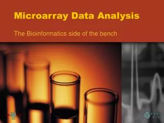
Microarray Data Analysis The Bioinformatics side of the bench
The anatomy of your data files from Affymetrix array analysis • .DAT= image file (107 pixels) • .CEL= measured cell intensities • .CHP= calculated probe set data
Quality Control (QC) of the chip – visual inspection • Look at the .DAT file or the .CHP file image • Scratches? Spots? • Corners and outside border checkerboard appearance (B2 oligo) • Positive hybridization control • Used by software to place grid over image • Array name is written out in oligos!
Internal controls • B. subtilis genes (added poly-A tails) • Assessment of quality of sample preparation • Also as hybridization controls • Hybridization controls (bioB, bioC, bioD, cre) • E. coli and P1 bacteriophage biotin-labeled cRNAs • Spiked into the hybridization cocktail • Assess hybridization efficiency • Actin and GAPDH assess RNA sample/assay quality • Compare signal values from 3’ end to signal values from 5’ end • ratio generally should not exceed 3 • Percent genes present (%P) • Replicate samples - similar %P values
Microarray Data Process/Outline • Experimental Design • Image Analysis – scan to intensity measures (raw data) • Normalization – “clean” data • More “low level” analysis-fold change, ANOVA, data filtering • Data mining-how to interpret > 6000 measures • Databases • Software • Techniques-clustering, pattern recognition etc. • Comparing to prior studies, across platforms? • Validation
Experimental Design A good microarray design has 4 elements • A clearly defined biological question or hypothesis • Treatment, perturbation and observation of biological materials should minimize systematic bias • Simple and statistically sound arrangement that minimizes cost and gains maximal information • Compliance with MIAME (minimal information about microarray experiment) • The goal of statistics is to find signals in a sea of noise • The goal of exp. design is to reduce the noise so signals can be found with as small a sample size as possible
Observational Study vs. Designed Experiment • Observational study- • Investigator is a passive observer who measures variables of interest, but does not attempt to influence the responses • Designed Experiment- • Investigator intervenes in natural course of events
Experimental Replicates • Why? • In any exp. system there is a certain amount of noise—so even 2 identical processes yield slightly different results • In order to understand how much variation there is it is necessary to repeat an exp a # of independent times • Replicates allow us to use statistical tests to ascertain if the differences we see are real
Technical vs. Biological Replicates As we progress from the starting material to the scanned image we are moving from a system dominated by biological effects through one dominated by chemistry and physics noise Within Affy platform the dominant variation is usually of a biological nature thus best strategy is to produce replicates as high up the experimental tree as possible
From probe level signals to gene abundance estimates The job of the MAS 5.0 expression summary algorithm is to take a set of Perfect Match (PM) and Mis-Match (MM) probes, and use these to generate a single value representing the estimated amount of transcript in solution, as measured by that probeset. To do this, .DAT files containing array images are first processed to produce a .CEL file, which contains measured intensities for each probe on the array. It is the .CEL files that are analyzed by the expression calling algorithm.
MAS 5.0 output files • For each transcript (gene) on the chip: • signal intensity • a “present” or “absent” call (presence call) • p-value (significance value) for making that call
How are transcripts determined to be present or absent? • Probe pair (PM vs. MM) intensities • generate a detection p-value • assign “Present”, “Absent”, or “Marginal” call for transcript • Every probe pair in a probe SET has a potential “vote” for presence call
PM and MM Probes • The purpose of each MM probe is to provide a direct measure of background and stray-signal (perhaps due to cross-hybridization) for its perfect-match partner. In most situations the signal from each probe-pair is simply the difference PM - MM. • For some probe-pairs, however, the MM signal is greater than the PM value; we have an apparently impossible measure of background.
MAS 5.0 gives a first level look at the data • MAS 5.0 does the calculations for you • .CHP file (presence call, p-value and expression signal). • Basic analysis in MAS 5.0, but it won’t handle replicates
Signal Intensity Across Chips • Other algorithms, ex. RMA, GCRMA, PLIER and others have been developed by academic teams to improve the precision and accuracy of signal calculations (no mismatch) and comparison across chips (normalization). • Import (.CEL) data into other software, Genesifter, GCOS, SpotFire, and many others. • In our Exp we will use Genesifter software and the RMA expression algorithm.
Normalization - “clean” data • “Normalizing” data allows comparisons ACROSS different chips • Intensity of fluorescent markers might be different from one batch to the other • Normalization allows us to compare those chips without altering the interpretation of changes in GENE EXPRESSION • Normalization is necessary to effectively make comparison between chips-and sometimes within a single chip.
Caveat… • There is NO standard way to analyze microarray data • Still figuring out how to get the “best” answers from microarray experiments • Best to combine knowledge of biology, statistics, and computers to get answers
Low level data processing is completed now what?Fold change, ANOVA, Data filtering
How do we want to analyze our data? • Pairwise analysis is most appropriate • Control vs. H2O2 • List of genes that are “up-regulated” or “down-regulated”
Where are we now? Through this analysis we now have a list of genes that we believe are differentially expressed. • Now what????
Higher LevelMicroarray data analysis • Clustering and pattern detection • Data mining and visualization • Linkage between gene expression data and gene sequence/function/metabolic pathways databases
Scatter plot of all genes in a simple comparison of two control (A) and two treatments (B: high vs. low glucose) showing changes in expression greater than 2.2 and 3 fold.
Types of Clustering • Herarchical • Link similar genes, build up to a tree of all • Self Organizing Maps (SOM) • Split all genes into similar sub-groups • Finds its own groups (machine learning)
Back to Biology • Do the changes you see in gene expression make sense BIOLOGICALLY? • If they don’t make sense, can you hypothesize as to why those genes might be changing? • Leads to many, many more experiments
The Gene Ontologies A Common Language for Annotation of Genes from Yeast, Flies and Mice …and Plants and Worms …and Humans …and anything else!
Gene Ontology Objectives • GO represents concepts used to classify specific parts of our biological knowledge: • Biological Process • Molecular Function • Cellular Component • GO develops a common language applicable to any organism • GO terms can be used to annotate gene products from any species, allowing comparison of information across species
Sriniga Srinivasan, Chief Ontologist, Yahoo! The ontology. Dividing human knowledge into a clean set of categories is a lot like trying to figure out where to find that suspenseful black comedy at your corner video store. Questions inevitably come up, like are Movies part of Art or Entertainment? (Yahoo! lists them under the latter.) -Wired Magazine, May 1996
The 3 Gene Ontologies • Molecular Function = elemental activity/task • the tasks performed by individual gene products; examples are carbohydrate binding and ATPase activity • Biological Process = biological goal or objective • broad biological goals, such as mitosis or purine metabolism, that are accomplished by ordered assemblies of molecular functions • Cellular Component= location or complex • subcellular structures, locations, and macromolecular complexes; examples include nucleus, telomere, and RNA polymerase II holoenzyme
Example: Gene Product = hammer Function (what)Process (why) Drive nail (into wood) Carpentry Drive stake (into soil) Gardening Smash roach Pest Control Clown’s juggling object Entertainment
Genome Overview and Statistics Gene Status Overview 25/08/06 27/02/07 Experimentally characterised (or published) 1560 (31.3%) 1607 (32.1)% Role inferred from homology 2433 (48.9%) 2329 (46.5)% Conserved protein (unknown biological role) 458 (9.2%) 572 (11.4) % S. pombe specific families 68 (1.4%) 47 (0.9)% Sequence orphan 403 (8.1%) 364 (7.3) % Dubious 57 (1.1%) 60 (1.2)%