Download
1 / 35
350 likes | 353 Views
Analyzing Redistribution Matrix with Wavelet. LI ZHU STATISTICS. Background. RMF is redistribution matrix function It is probability of observing a certain energy give the true energy; The dimension is very large(1078*1024)

E N D
Analyzing Redistribution Matrix with Wavelet LI ZHU STATISTICS
Background • RMF is redistribution matrix function • It is probability of observing a certain energy give the true energy; • The dimension is very large(1078*1024) • We take log transformation on RMF matrix, and we set 0 value in RMF as 10^-15 • We want to study the uncertainty of RMF matrix, or in the perfect case, find a way to simulate new RMF matrix!
Discrete wavelet decomposition cA3 cA2 Low Frequency cA1 cD3 sample cD2 High Frequency cD1
Coefficients vector X cA1 cD1 cA2 cD2 cA3 cD3 cA3 cD3 cD2 cD1
Basic method in modeling RMF • Use wavelet decomposition to get wavelet coefficients for each line of RMFs; • Construct multi-level model to model coefficients in each line. • Ideally, we will construct a hierarchical model to reduce the dimension of RMFs • Then we make Bayesian analysis to the model and get posterior draw of new RMFs wavelet coefficients • We can use inverse wavelet transformation to get simulated RMFs(we need to rescale to make sure row summation of each line is 1)
Wavelet decomposition Mean of coefficients Std of coefficients
More about coefficients Mean, cA3 Sd, cA3
More about coefficients Mean, cD3 Sd, cD3
More about coefficients Mean, cD2 Sd, cD2
More about coefficients Mean, cD1 Sd, cD1
Wavelet coefficient for 900 true energy • More than half coefficients are 0 • Only a very limited coefficients are significant greater than 0 • The position of non-zero part among 33 matrixes for a specific true energy are almost the same, which make the analyzing easier • We also have a very negative part.
Wavelet coefficient for 900 true energy • In the right graph, I plot coefficient of energy 900 among first 10 matrixes; • The shape of coefficients over the first 10 matrixes are almost the same; • Coefficients which are significant greater than 0 has larger variance; • The uncertainty of RMFs is now the uncertainty of wavelet coefficients; • The coefficients are closely correlated to each others;
Introduction of base function • We have seen for the same true energy, shape of wavelet coefficients are almost the same among 33 RMFs; • Among different true energies, the shape of wavelet coefficients are also similar, even though the position of the shape is different; • We may define the specific shape as base functions among all the true energies and matrixes.
Base function in RMF analysis • We may consider the base function a vector of size 1024 • The location where the base function is not equal to 0 is different for different true energies; • We may consider the location where base function is not equal to 0 for a specific true energy as a constant, not a parameter; • We won’t have too much base functions(around 10).
Example of base function • It will be a vector with dimension 1024, • Only the functional part(6~8elements) is different from 0; • For different true energy, the value of base function will be the same, except the location of elements which are different from 0.
The size of base function • For different true energy, the size of base function will be different; • The size of a base function among 1078 energies can be plotted as right; • We may use a regression model to model log size of base function(to make the variance a constant).
Naïve model after base function • After we define the base function, we may write the coefficients j for true energy i for matrix m as: • Coefficient(i,j,m)=size of base*base+error terms • We will have two kind of uncertainty in my model, uncertainty of value of base function and a noise on every coefficient.
Histogram of several coefficients 900 energy level • For every coefficients, we have 33 values; • Since they are random variables, we can plot the histogram of them • We can find the distribution are not quite normal; • Some relevant paper suggests some heavy-tail distribution to model the error;
Strong correlations between coefficients • The correlation between wavelet coefficients are very large; • If we do not consider the correlation and simulate independent error terms we will have very bad simulations; • We need to construct a model for the error terms;
Correlation between coefficients and the next coefficients on 900 true energy
Correlation between coefficients and the next coefficients on 600 true energy
Strong correlation error terms • In the graph, blue points are the correlation of coefficients and the next coefficients; • We can find we have very strong correlation between coefficients, especially the functional part; • We can also find variance structure between different true energies are very similar; • In the functional part, we can use a vector to model the correlation:
Correlation vector for functional part • The vector can model the variance and correlation structure of coefficient of base function; • For instance, if It means the first and second element of this base function will be highly negative correlated; For every base function, we will have a correlation vector.
Strong correlation error terms • For each nonzero part, we can consider it is an error term. • We can see from the previous slides the error terms are highly correlated. • For the error term, I suggest to use the following model to model error terms: • In this way, we can consider a and b as parameters and get the correlation. • for different part of the wavelet coefficient, we can assume are constant. • We can also construct hierachical models for a,b among different true energy.
My suggested model • We can consider a model in the following way: Coefficients(i,j,m)= base part + error part Base part= Error part:
Variance Term is sd for base function f and ith true energy; It is a function of true energy i, we can model them according to the variance plot; is sd for individually error terms. For different part of the coefficients, we can assume it is locally constant; is sd for each line, it can be considered as a function of true energy i is uncertainty for matrix.
Difficulty and challenge • Is it a good idea to use the base function, or do you have some suggestion? • Is there some other method to model the error terms in order to characterize the correlation? • The computation will be very intensive, is there some method to simply the model?
Further work • Computation of log-L with specific priors; • Use Bayesian method to draw posterior draw of new coefficients; • Use wavelet method to re-decompose new simulated RMFs; • Model checking and posterior checking;
Wavelet analysis of the error terms • In the dataset, we have 33 simulated RMFs and a default RMF • If we consider the default RMF as “true RMF”, we can get the difference between 33 RMFs and default RMF, which are the error terms • We may do wavelet analysis to the error terms and construct models to analysis them
Overall wavelet coefficients description • We use “db4” wavelet bases to do the analysis • Since this is the error terms, instead of original RMF, we won’t see too much original charactistic • We still take energy 900 as a example. • In the right graph, the blue points is mean for 33 RMF coefficients and red line indicates 2 standard deviation over 33 matrixes.
Rescaling factor • We can find large variance near channel 80, we can plot graph of 33 matrixes near channel 80 and energy 900; • However, if we can rescale the mode near 80, we can get the second graph; • We can still find the base function to deal with the problem. • For the other part, it is similar to the wavelet model part for original RMFs;