Download
1 / 27
300 likes | 431 Views
WAVELET TUTORIALS. FOURIER TRANSFORM (FT). Frequency-Amplitude representation of a signal. FT gives the frequency information of the signal, which means that it tells us how much of each frequency exists in the signal, but it does not tell us when in time these frequency components exist.

E N D
FOURIER TRANSFORM (FT) • Frequency-Amplitude representation of a signal • FT gives the frequency information of the signal, which means that it tells us how much of each frequency exists in the signal, but it does not tell us when in time these frequency components exist.
Example of Stationary Signal: x(t)=cos(2*pi*10*t)+cos(2*pi*25*t)+cos(2*pi*50*t)+cos(2*pi*100*t) • Is a stationary signal, because it has frequencies of 10, 25, 50, and 100 Hz at any given time instant. • Information regarding the time instant of occurance of a frequency is not required • FT of the signal shows spectrum with amplitudes to corresponding frequency
Example of Non Stationary Signal: • A signal whose frequency constantly changes in time • Signal with four different frequency components at four different time intervals, hence a non-stationary signal. • The interval • 0 to 300 ms = 100 Hz • 300 to 600 ms = 50 Hz • 600 to 800 ms = 25Hz • 800 to 1000 ms = 10 Hz sinusoid. • The FT has four peaks, corresponding to four frequencies with amplitudes.
Limitations of Fourier Transform: • FT is not a suitable technique for non-stationary signal, except if for non-stationary signals, we are only interested in what spectral components exist in the signal, but not interested where these occur. Inference: • When the time localization of the spectral components are needed, a transform giving the TIME-FREQUENCY REPRESENTATION of the signal is needed.
THE SHORT TERM FOURIER TRANSFORM (STFT) • The signal is divided into small enough segments, where these segments (portions) of the signal can be assumed to be stationary. • For this purpose, a window function "w" is chosen. The width of this window must be equal to the segment of the signal where its stationarity is valid. • STFT of the signal is nothing but the FT of the signal multiplied by a window function. For every t' and f a new STFT coefficient is computed
Computation of STFT: • Gaussian function are the windowing functions located at t=t1', t=t2' and t=t3'. These will correspond to three different FT’s at three different times. A true time-frequency representation (TFR) of the signal is obtained Example: STFT For the same non stationary signal
INFERENCE FROM STFT: • Consider the STFT, the "x" and "y" axes are time and frequency, respectively • Graph is symmetric with respect to midline of the frequency axis. FT of a real signal is always symmetric, since STFT is nothing but a windowed version of the FT the STFT is also symmetric in frequency. • There are four peaks corresponding to four different frequency components. Unlike FT, these four peaks are located at different time intervals along the time axis. Remember that the original signal had four spectral components located at different times.
THE UNCERTAINTY PRINCIPLE PROBLEM WITH STFT : • States that, we cannot exactly know what frequency exists at what time instance, but we can only know what frequency bands exist at what time • Only time intervals in which, certain band of frequencies exists is known pose a resolution problem influenced by window function • FT has no resolution problem in the frequency domain, since exp{jwt} function, lasts at all times from - to + (infinite length ) • STFT resolution is dependent on window which is of finite length
CASE STUDY FOR STFT: • Consider three windows of different length, and compute the STFT. • Window function is a Gaussian function in the form: • w(t)=exp(-a*(t^2)/2); • where ‘a’ determines the length of the window, and t is the time. Case I: • A most narrow window. • STFT having a very good time resolution, but relatively poor frequency resolution. • The four peaks are well separated from each other in time. In frequency domain, every peak covers a range of frequencies
CASE STUDY FOR STFT: Case II: • A wider window • Peaks are not well separated from each other in time • Frequency domain the resolution is much better. Case III: • Much wide window • Time resolution is totally lost
Conclusion from Case Study of STFT: • Narrow windows give good time resolution, but poor frequency resolution. • Wide windows give good frequency resolution, but poor time resolution • Wide windows may violate the condition of stationarity. • Choice of window function is application dependent. • Wavelet transform (WT) solves the dilemma of resolution to a certain extent
MULTIRESOLUTION ANALYSIS (MRA) • An alternative approach to analyze any signal regardless of Heisenberg uncertainty principle of the transform used. • Analyzes the signal at different frequencies with different resolutions. • Every spectral component is not resolved equally as was the case in the STFT • Designed to give good time resolution and poor frequency resolution at high frequencies (narrow window length) and good frequency resolution and poor time resolution at low frequencies (wide window length) • Signals in practical applications have high frequency components for short durations and low frequency components for long durations
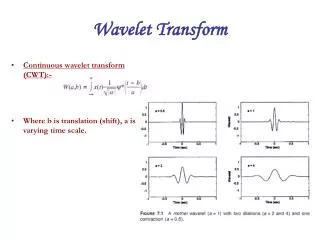
THE CONTINUOUS WAVELET TRANSFORM (CWT): • An alternative approach to overcome the resolution problem in STFT. • Wavelet means a small wave. The smallness refers to the condition that the window function is of finite length (compactly supported). The wave refers to the condition that this function is oscillatory. • Wavelet analysis is done in a similar way to the STFT in the sense that the signal is multiplied with a function similar to the window function in the STFT • Differences between the STFT and the CWT. • The Fourier transforms of the windowed signals are not taken, and therefore single peak will be seen corresponding to a sinusoid, i.e., negative frequencies are not computed. • The width of the window is changed as the transform is computed for every single spectral component, which is probably the most significant characteristic of the wavelet transform.
THE CONTINUOUS WAVELET TRANSFORM (CWT): • The continuous wavelet transform is defined as follows the transformed signal is a function of two variables, • = Translation s = Scale • (t) = Transforming function called the mother wavelet • Mother is a prototype for generating the other window functions which implies that the functions with different region of support that are used in the transformation process are derived from one main function. • Translation (same sense as in STFT) is related to the location of the window, as the window is shifted through the signal. This term, obviously, corresponds to time information in the transform domain. • Scale is defined as (1/frequency). • 1/s multiplication term is for energy normalization purposes so that the transformed signal will have the same energy at every scale.
The Scale (s): • Scaling, is a mathematical operation, either dilates or compresses a signal • High scales (low frequencies ) correspond to global information of a signal (that usually spans the entire signal) i.e., dilated signals, whereas low scales (high frequencies ) correspond to detailed information of a hidden pattern in the signal (that usually lasts a relatively short time) i.e., compressed signals. • compressed version of f(t) if s > 1 and an expanded (dilated) version of f(t) if s < 1 Wavelet Transform scaling term is used in the denominator, and hence opposite of the above statements holds, i.e., scales s > 1 dilates the signals whereas scales s < 1 , compresses the signal
COMPUTATION OF THE CWT • x(t) is the signal to be analyzed. • Mother wavelet is chosen the computation starts with s=1 and CWT is computed for all values of s, smaller and larger than 1. • Practical purposes, the signals are bandlimited, and therefore, computation of the transform for a limited interval of scales is usually adequate. • The analysis starts from high frequencies and proceed towards low frequencies. • The first value of s will correspond to the most compressed wavelet. As the value of s is increased, the wavelet will dilate. • Wavelet is placed in signal at t=0. The wavelet function at s=1 is obtained from the equation.
COMPUTATION OF THE CWT • The final result is CWT at t=0, s=1. or =0, s=1 in the time-scale plane. • The wavelet at scale s=1 is then shifted towards the right by amount to the location t=, and the above equation is computed to get the transform value at t=, s=1 in the time-frequency plane. • This procedure is repeated until the wavelet reaches the end of the signal. One row of points on the time-scale plane for the scale s=1 is now completed. • s is increased by a small value and process repeats.
Example: CWT For the same non stationary signal • For signal composed of four frequency components at 30 Hz (highest), 20 Hz, 10 Hz and 5 Hz (lowest). • WT has a good time and poor frequency resolution at high frequencies, and good frequency and poor time resolution at low frequencies
TIME AND FREQUENCY RESOLUTIONS (CWT): • Every box represents a value of WT in time-frequency plane. • Boxes have non-zero area implies value of a point in the time-frequency plane is not known. • All the points in the time-frequency plane that falls into a box represent one value of the WT • Widths and heights of the boxes change, the area is constant • Boxes represents an equal portion of the time-frequency plane, but giving different proportions to time and frequency • low frequencies, the height of the boxes are shorter (better frequency resolutions, less ambiguity regarding the value of the exact frequency), widths are longer (poor time resolution, more ambiguity regarding the value of the exact time). • At higher frequencies the width of the boxes decreases, i.e., the time resolution gets better, and the heights of the boxes increase, i.e., the frequency resolution gets poorer
Summarising… • The STFT case the representation in time-frequency plane consists of squares (constant window length). • Regardless of the dimensions of the boxes, the areas of all boxes, both in STFT and WT, are the same and determined by Heisenberg's inequality. • The area of a box is fixed for each window function (STFT) or mother wavelet (CWT), whereas different windows or mother wavelets can result in different areas. • All areas are lower bounded by 1/4pi the areas of the boxes cannot be reduced (due to the Heisenberg's uncertainty principle). • On the other hand, for a given mother wavelet the dimensions of the boxes can be changed, while keeping the area the same. This is exactly what wavelet transform does
THE WAVELET SYNTHESIS: The reconstruction is possible by using the equation C is a constant that depends on the wavelet used. The success of the reconstruction depends on this constant called, the admissibility constant, to satisfy the following admissibility condition where ^() is the FT of (t) and implies that ^() (0) = 0, which is hence the wavelet must be oscillatory for above equation to be satisfied.
THE DISCRETE WAVELET TRANSFORM (DWT) • SUBBAND CODING:Decompose discrete time signals • A time-scale representation of a digital signal is obtained using digital filtering techniques • CWT is a correlation between a wavelet at different scales and the signal with the scale (or the frequency) being used as a measure of similarity • DWT filters of different cutoff frequencies are used to analyze the signal at different scales • Let the discrete sequence be x[n], where n is an integer. Procedure starts with passing this signal (sequence) through a half band digital LPF with impulse response h[n]. Filtering a signal corresponds to the mathematical operation of convolution of the signal with the impulse response of the filter. The convolution operation in discrete time is defined as follows:
THE DISCRETE WAVELET TRANSFORM (DWT) • Low pass filtering halves the resolution, but leaves the scale unchanged.The signal is then subsampled by 2 since half of the number of samples are redundant. This doubles the scale. • The DWT analyzes the signal at different frequency bands with different resolutions by decomposing the signal into a coarse approximation and detail information. • DWT employs two sets of functions, called scaling functions and wavelet functions, which are associated with low pass h(n) and highpass filters g(n), respectively. where yhigh[k] and ylow[k] are the outputs of the highpass and lowpass filters, respectively, after subsampling by 2
Inverse DWT: The above procedure is followed in reverse order for the reconstruction. The signals at every level are upsampled by two, passed through the synthesis filters g’[n], and h’[n] (highpass and lowpass, respectively), and then added. Difficulties: If the filters are not ideal halfband, then perfect reconstruction cannot be achieved. Although it is not possible to realize ideal filters, under certain conditions it is possible to find filters that provide perfect reconstruction. The most famous ones are the ones developed by Ingrid Daubechies, and they are known as Daubechies’ wavelets
TYPES OF WAVELETS • Haar Wavelets • Shannon Wavelet • Meyer Wavelets • Daubechies Wavelets • Coifmann Wavelets APPLICATIONS OF THE WAVELETS Data processing Data compression Solution of differential equations