Download
1 / 43
430 likes | 519 Views
Polarization in Interferometry. Rick Perley (NRAO-Socorro). Apologies, Up Front. This is tough stuff. Difficult concepts, hard to explain without complex mathematics. I will endeavor to minimize the math, and maximize the concepts with figures and ‘handwaving’. Many good references:

E N D
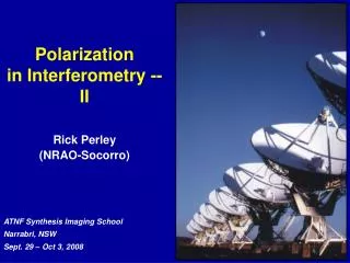
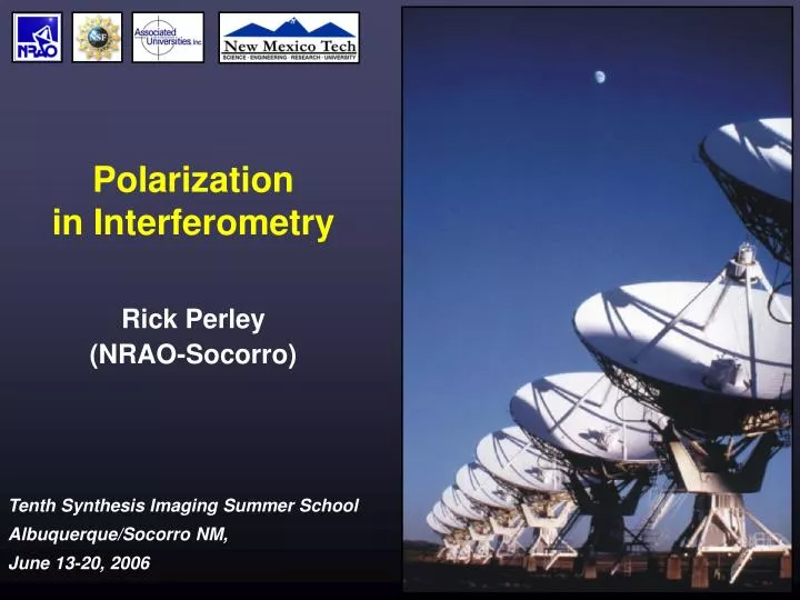
Polarization in Interferometry Rick Perley (NRAO-Socorro)
Apologies, Up Front • This is tough stuff. Difficult concepts, hard to explain without complex mathematics. • I will endeavor to minimize the math, and maximize the concepts with figures and ‘handwaving’. • Many good references: • Born and Wolf: Principle of Optics, Chapters 1 and 10 • Rolfs and Wilson: Tools of Radio Astronomy, Chapter 2 • Thompson, Moran and Swenson: Interferometry and Synthesis in Radio Astronomy, Chapter 4 • Tinbergen: Astronomical Polarimetry. All Chapters. • Great care must be taken in studying these – conventions vary between them. Polarization in Interferometry – Rick Perley
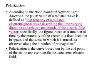
What is Polarization? • Electromagnetic field is a vector phenomenon – it has both direction and magnitude. • From Maxwell’s equations, we know a propagating EM wave (in the far field) has no component in the direction of propagation – it is a transverse wave. • The characteristics of the transverse component of the electric field, E, are referred to as the polarization properties. Polarization in Interferometry – Rick Perley
Why Measure Polarization? • In short – to access extra physics not available in total intensity alone. • Examples: • Processes which generate polarized radiation: • Synchrotron emission: Up to ~80% linearly polarized, with no circular polarization. Measurement provides information on strength and orientation of magnetic fields, level of turbulence. • Zeeman line splitting: Presence of B-field splits RCP and LCP components of spectral lines by by 2.8 Hz/mG. Measurement provides direct measure of B-field. • Processes which modify polarization state: • Faraday rotation: Magnetoionic region rotates plane of linear polarization. Measurement of rotation gives B-field estimate. • Free electron scattering: Induces a linear polarization which can indicate the origin of the scattered radiation. Polarization in Interferometry – Rick Perley
10 kpc Example: Cygnus A • VLA @ 8.5 GHz B-vectors Perley & Carilli (1996) Polarization in Interferometry – Rick Perley
Example: more Faraday rotation • See review of “Cluster Magnetic Fields” by Carilli & Taylor 2002 (ARAA) Polarization in Interferometry – Rick Perley
Example: Zeeman effect Polarization in Interferometry – Rick Perley
The Polarization Ellipse • By convention, we consider the time behavior of the E-field in a fixed perpendicular plane, from the point of view of the receiver. • For a monochromatic wave of frequency n, we write • These two equations describe an ellipse in the (x-y) plane. • The ellipse is described fully by three parameters: • AX, AY, and the phase difference, d = fY-fX. • The wave is elliptically polarized. If the E-vector is: • Rotating clockwise, the wave is ‘Left Elliptically Polarized’, • Rotating counterclockwise, it is ‘Right Elliptically Polarized’. Polarization in Interferometry – Rick Perley
Ellipticly Polarized Monochromatic Wave The simplest description of wave polarization is in a Cartesian coordinate frame. In general, three parameters are needed to describe the ellipse. The angle a = atan(AY/AX) is used later … Polarization in Interferometry – Rick Perley
Polarization Ellipse Ellipticity and P.A. • A more natural description is in a frame (x,h), rotated so the x-axis lies along the major axis of the ellipse. • The three parameters of the ellipse are then: Ah : the major axis length tan c = Ax/Ah: the axial ratio • : the major axis p.a. • The ellipticity c is signed: c > 0 => REP c < 0 => LEP Polarization in Interferometry – Rick Perley
Circular Basis • We can decompose the E-field into a circular basis, rather than a (linear) cartesian one: • where AR and AL are the amplitudes of two counter-rotating unit vectors, eR (rotating counter-clockwise), and eL (clockwise) • It is straightforwards to show that: Polarization in Interferometry – Rick Perley
Circular Basis Example • The black ellipse can be decomposed into an x-component of amplitude 2, and a y-component of amplitude 1 which lags by ¼ turn. • It can alternatively be decomposed into a counterclockwise rotating vector of length 1.5 (red), and a clockwise rotating vector of length 0.5 (blue). Polarization in Interferometry – Rick Perley
Stokes’ Parameters • The three parameters already defined (major axis p.a., ellipticity, and major axis length) are sufficient for a complete description of monochromatic radiation. • They have different units – a field amplitude, an angle, and a ratio. • It is standard in radio astronomy to utilize the parameters defined by George Stokes (1852): • Note that • Thus – a monochromatic wave is 100% polarized. Polarization in Interferometry – Rick Perley
Linear Polarization • Linearly Polarized Radiation: V = 0 • Linearly polarized flux: • Q and U define the plane of polarization: • Signs of Q and U tell us the orientation of the plane of polarization: Q > 0 U > 0 U < 0 Q < 0 Q < 0 U > 0 U < 0 Q > 0 Polarization in Interferometry – Rick Perley
Simple Examples • If V = 0, the wave is linearly polarized. Then, • If U = 0, and Q positive, then the wave is vertically polarized. • If U = 0, and Q negative, the wave is horizontally polarized. • If Q = 0, and U positive, the wave is polarized at pa = 45 deg • If Q = 0, and U negative, the wave is polarized at pa = -45. Polarization in Interferometry – Rick Perley
Q U Illustrative Examples – Thermal Emission from Mars U • Mars emits in the radio as a black body. • Shown are the I,Q,U,P images from Jan 2006 data at 23.4 GHz. • V is not shown – all noise. • Resolution is 3.5”, Mars’ diameter is ~6”. • From the Q and U images alone, we can deduce the polarization is radial, around the limb. • Position Angle image not usefully viewed in color. P I P Polarization in Interferometry – Rick Perley
Stokes Parameters • Why use Stokes parameters? • Tradition • They have units of power • They are simply related to actual antenna measurements. • They easily accommodate the notion of partial polarization of non-monochromatic signals. • We can (as I will show) make images of the I, Q, U, and V intensities directly from measurements made from an interferometer. • These I,Q,U, and V images can then be combined to make images of the linear, circular, or elliptical characteristics of the radiation. Polarization in Interferometry – Rick Perley
Non-Monochromatic Radiation, and Partial Polarization • Monochromatic radiation is a myth. • No such entity can exist (although it can be closely approximated). • In real life, radiation has a finite bandwidth. • Real astronomical emission processes arise from randomly placed, independently oscillating emitters (electrons). • We observe the summed electric field, using instruments of finite bandwidth. • Despite the chaos, polarization still exists, but is not complete – partial polarization is the rule. • Stokes parameters defined in terms of mean quantities: Polarization in Interferometry – Rick Perley
Stokes Parameters for Partial Polarization Note that now, unlike monochromatic radiation, the radiation is not necessarily 100% polarized. Polarization in Interferometry – Rick Perley
Antenna Polarization • To do polarimetry (measure the polarization state of the EM wave), the antenna must have two outputs which respond differently to the incoming elliptically polarized wave. • It would be most convenient if these two outputs are proportional to either: • The two linear orthogonal Cartesian components, (EX, EY) or • The two circular orthogonal components, (ER, EL). • Sadly, this is not the case in general. • In general, each port is elliptically polarized, with its own polarization ellipse, with its p.a. and ellipticity. • However, as long as these are different, polarimetry can be done. Polarization in Interferometry – Rick Perley
An Aside: Quadrature Hybrids • We’ve discussed the two bases commonly used to describe polarization. • It is quite easy to transform signals from one to the other, through a real device known as a ‘quadrature hybrid’. • To transform correctly, the phase shifts must be exactly 0 and 90 for all frequencies, and the amplitudes balanced. • Real hybrids are imperfect – an generate their own set of errors. 0 X R 90 90 Y L 0 Polarization in Interferometry – Rick Perley
Antenna Polarization Ellipse • We can thus describe the characteristics of the polarized outputs of an antenna in terms of its antenna polarization ellipse: cR and YR, for the RCP output cL and YL, for the LCP output If the antenna is equipped with circularly polarized feeds, • Or, cx and Yx, for the ‘X’ output, cY and YY, for the ‘Y’ output If the antenna is equipped with linearly polarized feeds. Polarization in Interferometry – Rick Perley
Four Independent Outputs • We are looking to determine the four Stokes values for the emission of interest. • We thus need four independent quantities from which we can derive I, Q, U, and V. • Each antenna provides two independent (differently polarized) outputs. • We thus generate four (complex) products for each pair of antennas, and ask: • How do these products relate to what we’re looking for? Polarization in Interferometry – Rick Perley
Four Complex Correlations per Pair • Two antennas, each with two differently polarized outputs, produce four complex correlations. • From these four outputs, we want to make four Stokes Images. Antenna 1 Antenna 2 R1 L1 R2 L2 X X X X RR1R2 RR1L2 RL1R2 RL1L2 Polarization in Interferometry – Rick Perley
Interferometer Response • DANGER! The next slide could be hazardous to your health! • We are now in a position to show the most general expression for the output of a complex correlator, comprising imperfectly polarized antennas to wide-band partially-polarized astronomical signals. • This is a complex expression (in all senses of that adjective), and I will make no attempt to derive, or even justify it. • The expression is completely general, valid for a linear system. Polarization in Interferometry – Rick Perley
Here it is! What are all these symbols? Rpq is the complex output from the interferometer, for polarizations p and q from antennas 1 and 2, respectively. Y and c are the antenna polarization major axis and ellipticity for states p and q. IV,QV, UV, and VV are the Stokes Visibilities describing the polarization state of the astronomical signal. Polarization in Interferometry – Rick Perley
Stokes Visibilities • And what (you ask), are the Stokes Visibilities? • They are the (complex) Fourier transforms of the I, Q, U, and V spatial distributions of emission from the sky. • IV I, QV Q, UV U, VV V • Thus, these are what we are looking to get from the four complex outputs from the baselines of the array. • Once we can recover the IV, QV, UV, and VV values from the complex interferometer response, we can invert them via a Fourier transform to obtain the four spatial images. Polarization in Interferometry – Rick Perley
Idealized Antennas • We now begin an analysis of this lovely expression. • To ease you in as painlessly as possible, let us consider the idealized situation where the antennas are perfectly polarized. • There are two cases of interest: Linear and Circular. Polarization in Interferometry – Rick Perley
Orthogonal, Perfectly Linear Feeds • In this case, c = 0, Yv = 0, YH = p/2. (We are presuming the antenna orientation is fixed w.r.t the sky). • Then, • From these, we can trivially invert, and recover the desired Stokes Visibilities. Polarization in Interferometry – Rick Perley
Perfectly Circular Antennas • So let us continue with our idealizations, and ask what the response is for perfectly circular feeds. • Now we have: cR = -p/4, cL = p/4. • Then, • And again a trivial inversion provides our desired quantities. Polarization in Interferometry – Rick Perley
Comments • I have assumed that the data are perfectly calibrated. In general, gain factors accompany each expression. • Examination of these expressions shows why in most cases, circularly polarized antennas are preferred: • Parallel-hand correlations of linear feeds are modulated by Q . As most of the compact sources we use for calibration are ~5% linearly polarized, but have no circular polarization, gain calibration is easier with circular feeds. • Derivation of Stokes Q for linear feeds requires subtraction of two large quantities, (Q = RVV – RHH) while for circular, it comes from the cross-hand response, (Q = RRL + RLR) which is independent of I. • From this simple analysis, circularly polarized feeds allow easier calibration, and more accurate measurement of linear polarization. Polarization in Interferometry – Rick Perley
Why not Circular for all? • The VLA (and EVLA) use circularly polarized feeds. • Most new arrays do not (e.g. ALMA, ATCA). • Do they know something we don’t? • Antenna feeds are natively linearly polarized. To convert to circular, a hybrid is needed. This adds cost, complexity, and degrades performance. • For some high frequency systems, wideband quarter-wave phase shifters may not be available, or their performance may be too poor. • Linear feeds can give perfectly good linear polarization performance, provided the amplifier/signal path gains are carefully monitored. • Nevertheless, the calibration issues remain, if linearly polarized calibrators are to be used. Polarization in Interferometry – Rick Perley
Alt-Az Antennas, and the Parallactic Angle • The prior expressions presumed that the antenna feeds are fixed in orientation on the sky. • This is the situation with equatorially mounted antennas. • For alt-az antennas, the feeds rotate on the sky as they track a source at fixed declination. • The angle between a line of constant azimuth, and one of constant right ascension is called the Parallactic Angle, h : where A is the antenna azimuth, f is the antenna latitude, and d is the source declination. Polarization in Interferometry – Rick Perley
Including Parallactic Angle variations • Presuming all antennas view the source with the same parallactic angle (not true for VLBI!), the responses from pure polarized antennas are straightforward to derive. • For Linear Feeds: Polarization in Interferometry – Rick Perley
Including Parallactic Angle variations • For circular polarized (rotating) feeds, the expressions are simpler: • For both systems, it is straightforward to recover the Stokes Visibilities, as • the parallactic angle is known. Polarization in Interferometry – Rick Perley
Imperfect (Elliptically Polarized) Antennas • So much for perfection. In the real world, we don’t get purely polarized antennas. How does reality modify our easy life? • We must now introduce the concept of the D-terms – an alternate description of antenna polarization. • These D-terms measure the departure of the antenna response from perfect circularity. • For well-designed systems, the magnitude of the Ds is small – typically .01 to .05. N.B.: The Y are in the antenna’s frame. Parallactic angle is removed. Polarization in Interferometry – Rick Perley
Interferometer Response, with the D-formulation • With this substitution, we can derive an alternate general form of the interferometer response: • Time for some approximations: |D| < .05, and |Q|, |U|, and |V| are both typically less than 5% of |I|. Thus, ignore all 2nd order products. Polarization in Interferometry – Rick Perley
‘Nearly’ Circular Feeds • We then get the much simpler set: • Our problem is now clear. The desired cross-hand responses are contaminated by a term of roughly equal size. • To do accurate polarimetry, we must determine these D-terms, and remove their contribution. Polarization in Interferometry – Rick Perley
Some Comments • If we can arrange that then there is no polarization leakage! (to first order). • This condition occurs if the two antenna polarization ellipses (R1 and L2 in the first case, and L1 and R2 for the second) have equal ellipticity and are orthogonal in orientation. • This is called the `orthogonality condition’. • Determination of the D (leakage) terms is normally done either by: • Observing a source of known (I,Q,U) strengths, or • Multiple observations of a source of unknown (I,Q,U), and allowing the rotation of parallactic angle to separate the two terms. • Note that for each, the absolute value of D cannot be determined – they must be referenced to an arbitrary value. Polarization in Interferometry – Rick Perley
Nearly Perfectly Linear Feeds • Sadly, the D-term formulation cannot be usefully applied to nearly-linear feeds, as the deviations from perfectly circularity are not small! • In the case of nearly-linear feeds, we return to the fundamental set, and assume that the ellipticity is very small (c << 1), and that the two feeds (‘dipoles’) are nearly perfectly orthogonal. • We then define a *different* set of D-terms: • The angles jH and jVare the angular offsets from the exact horizontal and vertical orientations, w.r.t. the antenna. Polarization in Interferometry – Rick Perley
This gives us … • I’ll spare you the full equation set, and show only the results after the same approximations used for the circular case are employed. Polarization in Interferometry – Rick Perley
Some Comments on Linears • The problem is the same as for the circular case – the derivation of the Q, U, and V Stokes’ visibilities is contaminated by a leakage of the much larger I visibility into the cross-hand response. • Calibration is similar to the circular case: • If Q, U, and V are known, then the equations can be solved directly for the Ds. • If the polarization is unknown, then the antenna rotation can again be used (over time) to separate the polarized response from the leakage response. Polarization in Interferometry – Rick Perley
A Summary (of sorts) • I’ll put something here, once I figure it all out! Polarization in Interferometry – Rick Perley