Download
1 / 35
360 likes | 551 Views
On the Closure of the Surface Energy Balance in Highly Complex Terrain. Mathias W. Rotach, Pierluigi Calanca, Andreas Weigel, Marco Andretta Swiss Federal Institute of Technology Institute for Atmospheric and Climate Science. Layout. Surface energy balance Data: MAP -Riviera project

E N D
On the Closure of the Surface Energy Balance in Highly Complex Terrain Mathias W. Rotach, Pierluigi Calanca, Andreas Weigel, Marco Andretta Swiss Federal Institute of TechnologyInstitute for Atmospheric and Climate Science
Layout • Surface energy balance • Data: MAP -Riviera project • Energy balance for a layer • Implications for modeling
MAP-Riviera Valley Floor Slope site Average 15 fair-weather days
Surface Energy balance NR-G=Ho+LvEo Ho LvEo NR G
Surface Energy balance NR-G=Ho+LvEo • horizontally homogeneous surfaces --> constant turbulent fluxes --> no advection-->closure! [even @ z≠0...]
Surface Energy balance NR-G=Ho+LvEo • horizontally homogeneous surfaces --> constant turbulent fluxes --> no advection-->closure! [even @ z≠0...]--> non-closure: measurement error turbulence time scales
Surface Energy balance NR-G=Ho+LvEo • horizontally homogeneous surfaces --> constant turbulent fluxes --> no advection-->closure! [even @ z≠0...]--> non-closure: measurement error turbulence time scalescomplex terrain...
MAP Riviera project Biasca Riviera Bellinzona Lago Maggiore
MAP-Riviera: Bosco di Sotto turbulence @ 4 / 16 / 28 m Full radiation comp, precip, profiles,sfc. hydrology Local slope app. 0.5° Local surface: corn, grass
Near-Surface Energy Balance H(zr) LvE(zr) NR zr Ho LvEo G
Near-Surface Energy Balance NR-G=Storage+horiz.Adv +vert.Adv Hr LvEr NR z=zr Ho LvEo G
Corrections • Sensible Heat flux:--> frequency response (Moore 1986) • --> humidity cross-correlation (Schotanus et al. 1983) • Latent heat flux: --> frequency response (Moore 1986) --> Oxygen (Dijk et al. 2003) • --> WPL-correction (Webb et al. 1980)
Horizontal Advection Comprovasco Riviera Magadino
Vertical Advection zr Mean vertical wind: from planar fit
Energy balance terms NR New sum H+LE+G LE H G Average 7 clear sky days
Contributing terms Sum new terms Vertical advection Sum corrections Storage soil Storage air / horiz. advection Average 7 clear sky days
Vertical advection Proprtional Difference in Q, q....
Vertical advection Proprtional mean vertical wind
Energy balance terms NR New sum H+LE+G LE H G Average 7 clear sky days
Conclusions • Sfc. energy balance in really complex terrain: good to detect processes • Corrections to turbulent fluxes important • Soil storage term important • Vertical advection!--> largest--> most uncertain!
Outlook • If indeed vertical advection is substantial....--> too large a fraction of NR --> H, LE--> cold / dry bias
RAMS simulations - August 25 1999 12.08 UTC 9.15 UTC observations model De Wekker et al. 2003
Salt Lake Valley - VTMX Different models: RAMSMM5ETA IOP‘s 6,7,10 Zhong and Fast 2002
Outlook • If indeed vertical advection is substantial....--> too large a fraction of NR --> H, LE--> cold / dry bias • How to parameterize in numerical models?
Hydrological modeling – valley floor ET und LE [mm/h] ET und LE [W/m2] Soil moisture (.5m) Precipitation [mm/h] Sept 1 1999 Sept 21 1999
Hydrological modeling – valley floor Observation(Bowen Ratio) Model (Penman- Monteith) ET und LE [W/m2] Eddy Correlation time
Closed energy balance • Bowen ratio method: --> if and
Planar fit Plot w as a function of (u,v)....
Planar fit vs. Double rotation Common plane vs. local planes (<u‘w‘>PFC -<u‘w‘>DR)/<u‘w‘>DR (<u‘w‘>PFC -<u‘w‘>PF)/<u‘w‘>PFC Andretta et al. (2002)
Energy Balance closure Data from a ‚flux site‘ in Manaus, Brazil Finnigan et al. 2003