Download
1 / 28
310 likes | 471 Views
Applying Machine Learning to Circuit Design. David Hettlinger Amy Kerr Todd Neller. Channel Routing Problems (CRPs). Chip Design Each silicon wafer contains hundreds of chips. Chip components, specifically transistors, are etched into the silicon.

E N D
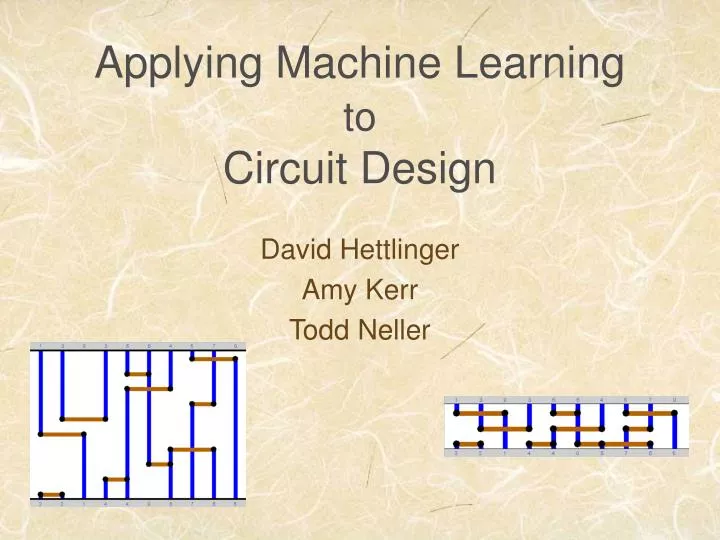
Applying Machine Learning toCircuit Design David Hettlinger Amy Kerr Todd Neller
Channel Routing Problems (CRPs) Chip Design • Each silicon wafer contains hundreds of chips. • Chip components, specifically transistors, are etched into the silicon. • Often groups of components need to be wired together.
3 4 1 0 2 4 Net number 4 4 2 0 3 1 2 A Simple CRP Instance Silicon Channel
3 4 1 0 2 4 0 1 2 3 4 5 4 2 0 3 1 2 One Possible Solution Goal: Decrease the number of horizontal tracks.
CRPs: Constraints • Horizontal: Horizontal segments cannot overlap. • Vertical : If subnet x has a pin at the top of column a, and subnet y has a pin at the bottom of column a, then subnet x must be placed above subnet y.
Simulated Annealing (SA) Background • “Annealing” came from a process blacksmiths use. • Metal is heated then cooled slowly to make it as malleable as possible. • Statistical physicists developed SA.
SA Problem Components • Definable states: The current configuration (state) of a problem instance must be describable. • New state generation: A way to generate new states. • Energy function: A formula for the relative desirability of a given state. • Temperature and annealing schedule: A temperature value and a function for changing it over time.
A Visual Example Local Minimum Global Minimum
Applying Simulated Annealing to CRPs • Definable states: The partitioning of subnets into groups. • New states generation: Change the grouping of the subnets. • Energy function: The number of horizontal tracks needed to implement a given partition. • Temperature and annealing schedule: Start the temperature just high enough to accept any new configuration. As for the annealing schedule, reinforcement learning can help find that.
A Simple CRP Example Start State of a CRP Instance Partition Graph of this State
A Simple CRP Example States 1 and 2 Partition Graphs of theses States
A Simple CRP Example States 1, 2 and 3 Partition Graphs of these States
A Simple CRP Example Starting through Ending States Partition Graphs of these States
A Generated CRP Instance Start State A Solution 12 Horizontal Tracks 15 Horizontal Tracks
SA Problem Components • Definable states: The current configuration (state) of a problem instance must be describable. • New state generation: A way to generate new states. • Energy function: A formula for the relative desirability of a given state. • Temperature and annealing schedule: A temperature value and a function for changing it over time.
The Drunken Topographer • Imagine an extremely hilly landscape with many hills and valleys high and low • Goal: find lowest spot • Means: airlift a drunk! • Starts at random spot • Staggers randomly • More tired rejects more uphill steps
Super-Drunks, Dead-Drunks, and Those In-Between • The Super-Drunk never tires • Never rejects uphill steps • How well will the Super-Drunk search? • The Dead-Drunk is absolutely tired • Always rejects uphill steps • How well will the Dead-Drunk search? • Now imagine a drunk that starts in fine condition and very gradually tires.
Traveling Salesman Problem • Have to travel a circuit around n cities (n = 400) • Different costs to travel between different cities (assume cost = distance) • State: ordering of cities (> 810865 orderings for 400 cities) • Energy: cost of all travel • Step: select a portion of the circuit and reverse the ordering
Determining the Annealing Schedule • The schedule of the “cooling” is critical • Determining this schedule by hand takes days • Takes a computer mere hours to compute!
Reinforcement Learning Example • Need to learn how long we need to study to get an A • Goal: Ace a class • Trial & Error: study for various amts. of time • Short term reward: exam grades, amt free time • Long term rewards: • Grade affects future opportunities: • i.e. whether we can slack off later • Our semester grades (goal is to max. this!)
Reinforcement Learning (RL) • Learns completely by trial & error • No preprogrammed knowledge • No human supervision/mentorship • Receives rewards for each action • 1. Immediate reward (numerical) • 2. Delayed reward: actions affect future • situations & opportunities for future rewards • Goal: maximize long-term numerical reward
RL: The Details Agent • Agent =the learner (i.e. the student) Sensation Reward Action Environment • Environment = everything the agent cannot completely control. • Includes reward functions (i.e. grade scale) • Descript. of current state (i.e. current average) • Call this description a “Sensation”
RL: Value Functions • Use immediate & delayed rewards to evaluate desirability of actions/learn task • Value function of a state-action pair, Q(s,a) • The expected reward for taking action a from state s • Includes immediate & delayed reward • Strategy: Most of the time, choose the action that corresponds to the maximal Q(s,a) value for the state. • Remember, must explore sometimes!
RL: Q-Functions • We must learn Q(s,a) • To start, set Q(s,a) = 0 for all s, a. • Agent tries various actions. • Each time experiences action a from state s, updates estimate of Q(s,a) towards the actual reward experienced • If usually pick the action a’ that has the maximal Q-value for that state • max. total reward optimal performance
Example: Grid World • Can always move up, down, right, left • Board wraps around • Get to goal in as few steps as • possible. • Reward = ? • Meaning of Q? • What are the optimal paths?
Applying RL to CRP • Can learn an approx. optimal annealing schedule using RL • Reward function: • Rewarded for reaching better configuration • Penalized for the amount of time used to find • this better configuration • Computer learns to find an approx optimal annealing schedule in a time-efficient manner. • Program self-terminates!
Conclusions • CRP is an interesting but complex problem • Simulated Annealing helps us solve CRPs • Simulated Annealing requires annealing schedule (how to change temperature over time) • Reinforcement learning – which is just learning through trial & error – lets a computer learn an annealing schedule in hours instead of days.