Download

1 / 36
360 likes | 554 Views
Overview of Numerical Models. Types of Atmospheric Models. Conceptual Norwegian Cyclone Model, Warm and Cold Fronts Analog and Pattern Pattern Recognition Statistical Stochastic, Gaussian Numerical Deterministic Models “First Principles” NWP, Case studies, Climate.

E N D
Types of Atmospheric Models • Conceptual • Norwegian Cyclone Model, Warm and Cold Fronts • Analog and Pattern • Pattern Recognition • Statistical • Stochastic, Gaussian • Numerical Deterministic Models “First Principles” • NWP, Case studies, Climate
Numerical ModelsDeterministic models based on the conservation laws of dynamics (hydrodynamics) and thermodynamics
Comparison of Human and Numerical Model Forecasting Method • Numerical • 1. Analysis or First Guess from previous run • 2. Data Assimilation , QC Data • 3. From 1 and 2 Establish Initial Conditions • 4 Time Step by numerically solving the dynamic and thermodynamic conservation equations that govern the atmosphere • Human 1. Analysis using Continuity (First Guess) 2. Non-standard Data Assimilation (Sat-Radar), QC Data 3. From 1 and 2 Establish Initial Conditions 4. Time Step using graphical techniques, conditional climatology, conceptual and theoretical models, empirical rules
Numerical Modeling System Components Interactive Models: Ocean, Hydrological Air Chemistry Terrain, Land Use, Soil Gridded Data Atmospheric Model Dynamical Core & Physics Computer Representation of E-A System Preprocessing Data Assimilation & Initialization INIT Output Gridded Databases Atmospheric Data Points and Grids Postprocessing and Visualization
TYPES OF NUMERICAL MODELSFinite Difference, Finite Element, Spectral Models, Adaptive Grids SCALES OF NUMERICAL MODELS GLOBAL REGIONAL GCM--- MRF----NGM---ETA---MASS/MM5---CLOUD Grid Spacing 300km--------100km------------20km------------1km YEARS---WEEKS-----DAYS-----DAY-----HOURS Macro/Synop----Mesoa-----Mesob----Mesog-----Micro
Nested runs from large to small scale Regional Models 2.5° x 2.5° NCEP Reanalysis Gridded Data
MODEL CONSIDERATIONSFree Atmosphere -Surface Energy-Radiation-PBL-Hydrology ATMOSPHERIC DATA INPUTGridded Data for Initial and LBCs, Observed via Data Assimilation PBL Terrain Hydrology Veg & LU Radiation SURFACE DATA INPUT DEEP SOIL MOISTURE/TEMP
. CONTINUE WRITE (6, 2025) DO 3310 KD=1,NZ CALL MXMIN2 (U(1,1,KD), NX,NY,NX,NY, . TMX,ITMX,JTMX, . TMN,ITMN,JTMN, . TAVG) WRITE (6, 2031) 'U-WIND COMP',KD, . TMX,ITMX,JTMX, . TMN,ITMN,JTMN, . TAVG
Relationship of Model Resolution, Observed Resolution, and Resolvable Features Model Spatial Avg 4 Grid Points Obs Only Valid at Point
Minimum Resolvable Feature Based Upon Grid Separation 0 5 10 15 20
Thoughts about Model Forecasts • Suppose there is an event where the MM5 or another model “nailed” precip forecast. • What must be true? • Parent model must have handled larger scale forcing because it provided initial and BC conditions • Any observed data assimilated into regional system was able to capture significant weather producing feature(s) • Mesoscale model was run at a grid spacing fine enough (horizontal and vertical) and had good enough dynamics and physics so was able to capture/ summate weather causing feature(s). • But can we really make this assertion?
Can you get the “right” answer for the “wrong” reason? • Example: Lake-Effect Snow Modeling : 15 km horizontal grid spacing, 30 levels. • Model does very good job depicting and forecasting lake- effect snow bands in central NY State. • Examine process. Model shows all precip is “Grid” scale (i.e., it was explicitly calculated, convective scheme was not turned on). Is this reasonable? • But Lake effect fundamentally a convective event. • So how can model do good job of positioning and QPF if model has fundamental problem simulating cause of precipitation? • That is, why it is doing poor job at depicting physical mechanism, but good job in forecasting precip.
Model is generating right answer for wrong reasons. • Two “mistakes” are offsetting one another. • In lake-effect case: • over production of vertical motion at grid scale • over abundance of latent heat • Over production of vertical motion incorrectly increases precip in region, but upper levels stabilized by over production of latent heat, decreasing precip, thus offsetting each other.
Why is this a problem for the operational meteorologist? • Because you are not always going to be so lucky to have these two factors offset each other for every parameter. • Ultimately the model will be go astray because it is heating the wrong levels.
Brazil Problem of Low Windspeeds Over ITCZ
Difference in mean annual 10 m wind speed between the MASS simulation of 365 days and 3 years of data from the TRMM Microwave imager (TMI)
Persistent Convergence zone Nearly continuous convection Identified Problem with Convective Radius Convective radius too large (1500 m) in K-F Reduced to 500 m What is unique about region of low wind bias?
Difference in mean annual 10 m wind speed between the MASS simulation of 365 days and 3 years of data from the TRMM Microwave imager (TMI) after trigger correction.
Identified Problem Number Two • NCAR-NCEP Reanalysis data too moist in upper levels along East coast of Brazil • NCAR-NCEP data used as initial and LB fields • Modified reanalysis data using satellite derived soundings
Difference in mean annual 10 m wind speed between the MASS simulation of 365 days and 3 years of data from the TRMM Microwave imager (TMI)
Difference in mean annual 10 m wind speed between the MASS simulation of 365 days and 3 years of data from the TRMM Microwave imager (TMI)
Current Model Limitations • Quality and availability of initialization data • Both surface and atmospheric • Limitations of numerical methods because of computational and resolution issuesand need to parameterize processes • Lack of understanding of processes