Download
1 / 58
580 likes | 719 Views
Radiation transfer in numerical models of the atmosphere. Jean-Jacques Morcrette adapted for presentation at KNMI by Erik van Meijgaard. Lectures. First hour: Introduction Radiation Transfer in the atmosphere: Basic concepts and approximations Second hour:

E N D
Radiation transfer in numerical models of the atmosphere Jean-Jacques Morcrette adapted for presentation at KNMI by Erik van Meijgaard
Lectures • First hour: • Introduction • Radiation Transfer in the atmosphere: Basic concepts and approximations • Second hour: • The ECMWF shortwave and longwave radiation schemes • Call Tree Radiation Scheme
References • Liou, K.-N., 1992: Radiation and Cloud Processes in the Atmosphere. Oxford University Press, 487 pp. • Liou, K.-N., 1980: An Introduction to Atmospheric Radiation. International Geophysics Series, Vol. 25, Academic Press, 392 pp. • Fouquart, Y., 1987: Radiative transfer in climate models. NATO ASI May 1986, M.E. Schlesinger, Ed., Kluwer Academic Publ., 223-284. • Goody, R.M., and Y.L. Yung, 1989: Atmospheric Radiation - Theoretical basis, 2nd ed., Oxford University Press. • Morcrette et al., 2007: Technical Memo 539, and JGR-Atm, Dec’2008
Outline of Introduction • Need for parametrisation • Global energy balance • Time and space variations of the solar zenith angle • A Top of the Atmosphere (ToA) view of the components of the Earth’s radiative budget
The parametrisation problem - 1 Adiabatic processes Cloud Fraction Cloud Water Humidity Temperature Winds Cumulus convection Stratiform precipitation Radiation Diffusion Evaporation Sensible heat flux Friction Ground humidity Snow Ground temperature Ground roughness Snow melt
The parametrisation problem - 2 • Assumption • Horizontal radiative fluxes are negligible (Independent Column Approximation) so vertical profile of radiative fluxes can be computed from local vertical distributions of the relevant parameters as well as the boundary conditions at the surface and top of the atmosphere
The parametrisation problem - 3 • In the ECMWF model, the 3-D distributions of T, H2O, cloud fraction (CF), cloud liquid water (CLW), cloud ice (CIW) are given for every time-step by the prognostic equations. • Other parameters, i.e., O3, CO2 and other uniformly mixed gases of radiative importance (O2, CH4, N2O, CFC-11, CFC-12 and aerosols) have to be specified (prognostic O3 soon interactive with rad?). • Prognostic aerosols (as part of GEMS project) to be used in the thermodynamic equation Radiation black box Profiles of T, q, CF, CLW, CIW, O3 OUTPUT updated from time to time Efficient radiation transfer algorithms DFLW, DFSW to be used in the surface (soil) energy balance equation Climatological data: other trace gases, aerosols
Radiation and the general circulation - 1 • What is the time scale? • (traditionally) Large characteristic time scale (but for clear-sky and the stratosphere). Radiation within stratosphere ~ 50-120 days • 10 to 20 times slower than effects of other physical processes Since the main part of the atmosphere (troposphere - stratosphere ?) is far away from state of radiative equilibrium, radiative effects (which are permanent) are generally cumulative and therefore non negligible. They also occur everywhere (NP to SP, surface to ToA). Of course, there are feedbacks! Those between clouds and radiation have a time scale similar to that of the cloud processes, and are therefore much faster.
Radiation and the general circulation - 2 • Differences with other physical processes • There exists a well known theory (from Quantum Mechanics to Spectroscopy to Radiation Transfer). • Radiation is exchanged with the outside space: radiative balance determines the climate. • The sun providing the energy input, radiation undergoes regular forcings: seasonal, diurnal. • Radiation at ToA has been globally measured since the 60’s (by operational satellites), with real flux measurements from ERB (1978), ERBE (1985), ScaRaB (1993), CERES (1998). • Surface radiation has been (roughly) measured at points over almost 40 years. Present programs like ARM, BSRN, SURFRAD measure it with high accuracy. Also satellite-derived SW (and LW) radiation is becoming available. • Therefore, there exist some relatively extended possibilities of validation/verification (radiation in the SW visible and near-IR, in the LW, … in the mW).
The global radiative balance - 1 S Difference with actual surface temperature Ts (=288 K) is due to the GREENHOUSE EFFECT: The atmosphere is (almost) transparent in the shortwave range (0.2 - 4.0 mm), and more opaque in the longwave range (4-100 mm) => there exists a temperature gradient between the surface and the ToA S = 1370+/- 4 Wm-2 dm = 1.5 +/- 0.03 1011 m Earth as a black body would give p R2 S = 4p R2s Tg4 => Tg = 278 K Earth with an actual albedo a = 0.30 p R2 S (1-a) = 4 p R2 s Te4 => Te = 255 K
The global radiative balance - 2 Solar 237 Terrestrial 343 Latent heat Sensible heat 237 H2O, CO2, O3, ... All fluxes in Wm-2 68 106 390 atmosphere 327 90 169 16
Time and space variations of the solar zenith angle - 1 qo = f( latitude, longitude day of the year, time of the day) mo = cos ( qo ) qo Two influences: - amount of energy incident at ToA above of given point of the Earth S = So ( d / dm )2m0 - the atmospheric mass encountered by a solar beam is proportional to 1 / m0 => Need to account for the daily cycle, and the yearly seasonal cycle
Time and space variations of the solar zenith angle - 2 • Implications • Better insolation of the equatorial belt than of polar regions (not compensated by the terrestrial/thermal/longwave output) • => equatorial regions are warmer than the polar ones • => same pressure layers are thicker at Equator than at the poles • => since sea level pressure is uniformised by friction in the PBL, given the rotation of the Earth and Buys-Ballot’s law, there should be westerlies • => there is a need to transport heat from Equator to polar regions • oceanic transport • disturbances in the zonal mean flow
Time and space variations of the solar zenith angle - 3 • Implications for modelling • In the tropics, the maximum net SW heating of 50 to 60 Wm-2 is only about 20% of the total absorbed SW radiation. • The other 80% contributes to the warming of the tropical surface, which in turn radiates the energy back to space in terms of LW radiation. • Therefore, any systematic error on the determination of the SW column net heating in the tropics can potentially induce an error 5 times larger in the required poleward transport of heat (by the ocean and the atmosphere) • If SST is specified, the whole error goes into the atmospheric contribution, with direct impact on the atmospheric structure, the stability, and the resultant convection (intensity and temporal characteristics)
A Top-of-the-Atmosphere view Outgoing Longwave Radiation: OLR Inter Tropical Convergence Zone: high-level cloudiness: Tcloud << Tsurf I Subtropics: clear-sky or low-level cloudiness Polar latitudes: Tcloud not very different from Tsurf Clear-sky OLR obtained by averaging over the clear-sky situations (based on thresholds) Permanent cloudiness
A Top-of-the-Atmosphere view Absorbed Shortwave Radiation ASW = Sxy ( 1 - axy ) ITCZ Highly reflecting stratocumulus cloud decks are seen in the SW, not in the LW ASW: Absorption Short Wave REF: Reflectance Short Wave CSREF: Clear Sky REF
A Top-of-the-Atmosphere view Cloud forcing: Total - Clear-Sky In the SW: ASWtotal - ASW clear-sky is negative: Clouds cool the atmosphere-surface system In the LW: OLRtotal - OLR clear-sky is generally positive: Clouds heat the atmosphere-surface system Clouds show large SW and LW cloud forcing in the tropics, which largely cancel out. Overall |SWCF| > |LWCF|, clouds have a cooling effect. Narrow FOV: Narrow Field of View SWCF/LWCF: Cloud Forcing
The basics - 0 • Definitions • The Radiative Transfer Equation (RTE) • The relevant laws • Planck’s • Wiens’s • Stefan-Boltzmann • Kirchhoff’s • A bit of useful spectroscopy • Line width (Lorentz, Doppler) • Line intensity
L. Boltzmann J. Stefan M. Planck W. Wien H.A. Lorentz C. Doppler G. Kirchhoff
The basics – Definitions 1 • Units • wavelength l (m), frequency n (Hz), wavenumber (m-1) • F flux density W m-2 flux per unit area, flux or irradiance • L specific intensity W m-2 sr-1 flux per unit area into unit solid, radiance • Solar / Shortwave spectrum • ultraviolet: 0.2 - 0.4 mm • visible: 0.4 - 0.7 mm • near-infrared: 0.7 - 4.0 mm • Infrared / Longwave spectrum • 4 - 100 mm C = 2.99793 x 10⁸ m s-1
The basics - 2 • The Radiative Transfer Equation (RTE) • For GCM/RCM/SCM applications, • no polarization effect • stationarity (no explicit dependence on time) • plane-parallel (no sphericity effect) • Sources and sinks: • Extinction • Emission • Scattering
The basics - RTE 1 • Extinction • Radiance Ln(z, q, f) entering the cylinder at one end is extinguished within the volume (negative increment) • bn,ext is the monochromatic extinction coefficient (m-1) • dw is the solid angle differential • dl the length • da the area differential
The basics - RTE 2 • Emission • b n,abs is the monochromatic absorption coefficient (m-1) • Bn(T) is the monochromatic Planck function
The basics - RTE 3 • Scattering • change of radiative energy in the volume caused by scattering of radiation from direction (q’,f’) into direction (q,f) • b n,scat is the monochromatic scattering coefficient • dw’ is the solid angle differential of the incoming beam • Pn(z,q,f,q’,f’) is the normalized phase function, I.e., the probability for a photon incoming from direction (q’,f’) to be scattered in direction (q,f), with
The basics - RTE 4 • Since scattered radiation may originate from any direction, need to integration over all possible (q’,f’) • The direct unscattered solar beam is generally considered separately • Eon is the specific intensity of the incident solar radiation • (qo,fo) is the direction of incidence at ToA • mo is the cosine of the solar zenith angle • dn is the optical thickness of the air above z
The basics - RTE 5 • The optical thickness is given by • The total change in radiative energy in the cylinder is the sum, and after replacing dl by the geometrical relation • considering that • and introducing the single scattering albedo
The basics - RTE 6 • The most general expression of the radiative transfer equation is
The basic laws - 1 • Planck’s law • for one atomic oscillator, change of energy state is quantized • for a large sample, Boltzmann statistics (statistical mechanics) • NB: h is Planck’s constant 6.626 x 10⁻³⁴ Js k is Boltzmann’s constant 1.381 x 10⁻²³ JK-1 c is the speed of light in a vacuum 2.9979 m s-1
The basic laws - 2 • Wien’s law • extremes of the Planck function are defined by • Stefan Boltzmann’s law • Kirchhoff’s law: in thermodynamic equilibrium, i.e., up to ~50-70 km depending on gases emissivity el = absorptivity al c1=2hc2 c2=hc/k x=c2/(lT) l5=c25 /(x5T5) lmax Tmax = 2897 mm K F = pB(T) = sT4
The basic laws - 3 • Spectral behaviour of the emission/absorption processes • Planck function has a continuous spectrum at all temperatures • Absorption by gases is an interaction between molecules and photons and obeys quantum mechanics • kinetic energy: not quantized ~ kT/2 • quantized:changes in levels of energy occur by DE=h Dn steps • rotational energy: lines in the far infrared l > 20mm • vibrational energy (+rotational): lines in the 1 - 20 mm • electronic energy (+vibr.+rot.): lines in the visible and UV
The basic laws - 4 • Line width • In theory and lines are monochromatic • Actually, lines are of finite width, due to natural broadening (Heisenberg’s principle) • Doppler broadening due to the thermal agitation of molecules within the gas: from a Maxwell-Boltzmann probability distribution of the velocity • the absorption coefficient of such a broadened Doppler line is • with
The basic laws - 5 • Line width • Pressure broadening (Lorentz broadening) due to collisions between the molecules, which modify their energy levels. The resulting absorption coefficient is • with the half-width proportional to the frequency of collisions
The basic laws - 4 • Line intensity E is the energy of the lower state of the transition x is an exponent depending on the shape of the molecule 1 for CO2, 3/2 for H2O, 5/2 for O3 T0 is the reference temperature at which the line intensities are known
Approximations - 0 • What is required in any RT scheme? • Transmission function • band model • scaling and Curtis-Godson approximations • correlated-k distribution • Diffusivity approximation • Scattering by particles
Approximations - 1 • What is required to build a radiation transfer scheme for a GCM? • 5 elements, the last, in principle in any order: • a formal solution of the radiation transfer equation • an integration over the vertical, taking into account the variations of the radiative parameters with the vertical coordinate • an integration over the angle, to go from a radiance to a flux • an integration over the spectrum, to go from monochromatic to the considered spectral domain • a differentiation of the total flux w.r.t. the vertical coordinate to get a profile of heating rate
Approximations - 2 • Band models of the transmission function over a spectral interval of width Dn • Goody • Malkmus are the mean intensity and the mean half-width of the N lines within Dn, with mean distance between lines d
Approximations - 3 • Mean line intensity • Mean half-width
Approximations - 4 • In order to incorporate the effect of the variations of the b n,x coefficients with temperature T and pressure p • Scaling approximation The effective amount of absorber can be computed with x,y coefficients defined spectrally or over the whole spectrum
Approximations - 5 • 2-parameter or Curtis-Godson approximation All these parameters can be computed from the information, i.e., the Si , ai , included in spectroscopic database like HITRAN
Approximations - 6 • Correlated-k distribution (in this part ki=bn,abs) • ki, the absorption coefficient shows extreme spectral variation. • Computational efficiency can be improved by replacing the integration over l with a reordered grouping of spectral intervals with similar ki strength. • The frequency distribution is obtained directly from the absorption coefficient spectrum by binning and summing intervals Dnj which have absorption coefficient within a range ki and ki+Dki • The cumulative frequency distribution increments define the fraction of the interval for which kv is between ki and ki+Dki Lacis, A.A. and V. Oinas, 1991: J.Geophys.Res., 96D, 9027-9063.
Approximations - 7 • The transmission function, over an interval [n1,n2], can therefore be equivalently written as
Approximations - 8 • Diffusivity factor • a flux is obtained by integrating the radiance L over the angle • with the transmission in the form • the exact solution involves the exponential integral function of order 3 where r ~ 1.66 is the diffusivity factor