Download
1 / 18
180 likes | 284 Views
Artificial deadtime Optimization for the - SN- system 2.0. Timo Griesel IceCube Collaboration Meeting 09/15-09/19/2008 Utrecht, Netherlands. Correlated Noise. __________________________________________________. __________________________________________________.

E N D
ArtificialdeadtimeOptimizationforthe - SN-system 2.0 Timo Griesel IceCube Collaboration Meeting 09/15-09/19/2008 Utrecht, Netherlands
Correlated Noise __________________________________________________ __________________________________________________ Time betweentwohits DOM 754dad1d3800 (Str49-1) Ideal poissoniannoise Correlatednoise, Afterpulses Shown fit : Page 1/15 Timo Griesel, I3Collaboration Meeting, Utrecht 2008
Dependancies: Correlated Noise __________________________________________________ __________________________________________________ Extraction of the temperature values from moni_histo_110352.root … looks like the correlation is depth and therefor temperature dependent … Page 2/15 Timo Griesel, I3Collaboration Meeting, Utrecht 2008
Temperaturedependance __________________________________________________ __________________________________________________ Correlated noise rises with falling temperature Not thermal noise fit: Mayer arXiv:0805.0771v1 Page 3/15 Timo Griesel, I3Collaboration Meeting, Utrecht 2008
The optimization method Generating SN Signal NSN Superpose NSN with measured background NB Apply artificial deadtime to the sample NSN+B Apply artificial deadtime to the sample NB Significance Increase artificial deadtime __________________________________________________ __________________________________________________ Page 4/15 Timo Griesel, I3Collaboration Meeting, Utrecht 2008
The supernova signal __________________________________________________ __________________________________________________ Two different SN signals were used (e.g. @ 10kpc): (1.) Scaled SN1987A signal (2.) SN signal based on the „Mainz Simulation“ (A.Piégsa & T.Griesel) Page 5/15 Timo Griesel, I3Collaboration Meeting, Utrecht 2008
Significance DOMs Str49 __________________________________________________ __________________________________________________ Scaled SN1987A signal @ distance 10kpc, String 49 Page 6/15 Timo Griesel, I3Collaboration Meeting, Utrecht 2008
Significance DOMs Str49 __________________________________________________ __________________________________________________ Scaled SN1987A signal @ distance 10kpc, String 49 Is it possible to use all DOMs on string ? Page 7/15 Timo Griesel, I3Collaboration Meeting, Utrecht 2008
The deadtimeoptimum __________________________________________________ __________________________________________________ Ideal deadtime Str49 & Str39 Page 8/15 Timo Griesel, I3Collaboration Meeting, Utrecht 2008
The optimizationmethod – a new Ansatz __________________________________________________ __________________________________________________ Azriel Goldschmidt suggested a different „counting sceme“ n=2 n=5 t t Significance is 16% higher ! Page 9/15 Timo Griesel, I3Collaboration Meeting, Utrecht 2008
Howfarcanwelook ? __________________________________________________ __________________________________________________ Dwf@20.0kpc LMC@48.1kpc SMC@60.6kpc Karachentsev et al. AJ 127:2031-2068, 2004 Macci et al. AJ 652:1133-1149, 2006 Holland et al. AJ 115:1916-1920, 1998 Page 10/15 Timo Griesel, I3Collaboration Meeting, Utrecht 2008
Howfarcanwelook ? __________________________________________________ __________________________________________________ Dwf@20.0kpc LMC@48.1kpc SMC@60.6kpc Karachentsev et al. AJ 127:2031-2068, 2004 Macci et al. AJ 652:1133-1149, 2006 Holland et al. AJ 115:1916-1920, 1998 Page 11/15 Timo Griesel, I3Collaboration Meeting, Utrecht 2008
Howfarcanwelook ? __________________________________________________ __________________________________________________ SNI3Daq triggers SNEWS alarm at a significance of 6.1 Page 12/15 Timo Griesel, I3Collaboration Meeting, Utrecht 2008
No. of Afterpulses __________________________________________________ __________________________________________________ All based on the assumption that „real hits“ have less or no afterpulses … is that true ? = 0µs = 150µs = 200µs = 250µs Page 13/15 Timo Griesel, I3Collaboration Meeting, Utrecht 2008
LocalCoincidenceevents __________________________________________________ __________________________________________________ Reprocessing the data to tag LC events Constraint for tagging a hit on DOM B as LC hit: A Probability to tag an accidental LC hit: B ~ 1% of the noise hits are LC hits: C Effectivescatteringcoefficientdata was providedbyWoschnagg Page 14/15 Timo Griesel, I3Collaboration Meeting, Utrecht 2008
LocalCoincidenceevents – No. ofafterpulses __________________________________________________ __________________________________________________ = 0µs = 150µs = 200µs = 250µs LC events have afterpulses !!! Page 15/15 Timo Griesel, I3Collaboration Meeting, Utrecht 2008
LocalCoincidenceevents __________________________________________________ __________________________________________________ In case an LC hit occurs: data was taken in SLC mode, this leads to an intrinsic deadtime LC hits found by our algorithm, which were not acquired as SLC hits Correlated hits due to drifting ions in the PMT longest cable length correction used + LC post window + 5 clock cycles + 2 clock cycles to arm the second ATWD = 1325ns + 1000ns + 5 * 25ns + 2 * 25ns = 2500ns When a data acquisition is in progress, the second Data Acquisition Channel will not get launched while the FADC still acquires data (6.4μs) Page 15/15 Timo Griesel, I3Collaboration Meeting, Utrecht 2008
LocalCoincidenceevents __________________________________________________ __________________________________________________ Scaled LC and Noise time differences „Real Events“ have less afterpulses than „noise“ events !!!!! Page 15/15 Timo Griesel, I3Collaboration Meeting, Utrecht 2008