Download
1 / 31
310 likes | 435 Views
Data Warehousing and Decision Support, part 3. CS634 Class 24, May 5, 2014. Slides based on “Database Management Systems” 3 rd ed , Ramakrishnan and Gehrke , Chapter 25. Partition Pruning. The QP needs to be smart about partitions/MDC cells

E N D
Data Warehousing and Decision Support, part 3 CS634Class 24, May 5, 2014 • Slides based on “Database Management Systems” 3rded, Ramakrishnan and Gehrke, Chapter 25
Partition Pruning • The QP needs to be smart about partitions/MDC cells • From Oracle docs, the idea: “Do not scan partitions where there can be no matching values”. • Example: partitions of table t1 based on region_code: PARTITION BY RANGE( region_code ) ( PARTITION p0 VALUES LESS THAN (64), PARTITION p1 VALUES LESS THAN (128), PARTITION p2 VALUES LESS THAN (192), PARTITION p3 VALUES LESS THAN MAXVALUE ); Query: SELECT fname, lname, region_code, dob FROM t1 WHERE region_code > 125 AND region_code < 130; • QP should prune partitions p0 (region_code too low) and p3 (too high). • But the capability is somewhat fragile in practice.
Partition Pruning is fragile • From dba.stackexchange.com: • The problem with this approach is that partition_year must be explicitly referenced in queries or partition pruning (highly desirable because the table is large) doesn't take effect. (Can’t ask users to add predicates to queries with dates in them) • Answer: • … Your view has to apply some form of function to start and end dates to figure out if they're the same year or not, so I believe you're out of luck with this approach. • Our solution to a similar problem was to create materialized views over the base table, specifying different partition keys on the materialized views. • So need to master materialized views to be an expert in DW.
Parallelism is essential to huge DWs • Table 1: Parallelism approaches taken by different data warehouse DBMS vendors, from “How to Build a High-Performance Data Warehouse” by David J. DeWitt, Ph.D.; Samuel Madden, Ph.D.; and Michael Stonebraker, Ph.D. • (I’ve added bold for the biggest players, green for added entries)
Views and Materialized Views Views: review of pp. 86-91 View- rows are not explicitly stored, but computed as needed from view definition Base table - explicitly stored
CREATE VIEW Given tables for these relations: Students (ID, name, major) Enrolled (ID, CourseID, grade) Can create view: CREATE VIEW B_Students(name, ID, CourseID) AS SELECT S.name, S.ID, E.CourseID FROM Students S, Enrolled E WHERE S.ID = E.ID AND E.grade = ‘B’; • Now can use B_Students just as if it were a table, for queries • Could be used to shield D_students from view • Can grant select on view, but not on enrolled
Updatable Views SQL-92: Must be defined on a single table using only selection and projection and not using DISTINCT. SQL:1999: May involve multiple tables in SQL:1999 if each view field is from exactly one underlying base table and that table’s PK is included in view; not restricted to selection and project, but cannot insert into views that use union, intersection, or set difference. So B_Students is updatable by SQL99, and by Oracle 10.
Materialized Views • What is a Materialized View? • Advantages and Disadvantages • Creating Materialized Views • Syntax, Refresh Modes/Options, Build Methods • Examples • Dimensions • What are they? • Examples • Slides of Willie Albino from http://www.nocoug.org/download/2003-05/materialized_v.ppt Willie Albino May 15, 2003
What is a Materialized View? • A database object that stores the results of a query • Features/Capabilities • Can be partitioned and indexed • Can be queried directly • Can have DML applied against it • Several refresh options are available (in Oracle) • Best in read-intensive environments Willie Albino May 15, 2003
Advantages and Disadvantages • Advantages • Useful for summarizing, pre-computing, replicating and distributing data • Faster access for expensive and complex joins • Transparent to end-users • MVs can be added/dropped without invalidating coded SQL • Disadvantages • Performance costs of maintaining the views • Storage costs of maintaining the views Willie Albino May 15, 2003
Similar to Indexes • Designed to increase query Execution Performance. • Transparent to SQL Applications allowing DBA’s to create and drop Materialized Views without affecting the validity of Applications. • Consume Storage Space. • Can be Partitioned. • Not covered by SQL standards • But can be queried like tables
MV Support in DBs: from Wikipedia • Materialized views were implemented first by the Oracle , and Oracle has the most features • In IBM DB2, they are called "materialized query tables"; • Microsoft SQL Server has a similar feature called "indexed views". • MySQL doesn't support materialized views natively, but workarounds can be implemented by using triggers or stored procedures or by using the open-source application Flexviews.
Views vs Materialized Views (Oracle), from http://www.sqlsnippets.com/en/topic-12874.html
Materialized View Logs for fast refresh • There is a way to refresh only the changed rows in a materialized view's base table, called fast refreshing. • For this, need a materialized view log (MLOG$_T here) on the base table t: create materialized view log on t ; UPDATE t set val = upper( val ) where KEY = 1 ; INSERT into t ( KEY, val ) values ( 5, 'e' ); select key, dmltype$$ from MLOG$_T ; KEY DMLTYPE$$ ---------- ---------- 1 U 5 I
REFRESH FAST create materialized view mv REFRESH FAST as select * from t ; select key, val, rowid from mv ; KEY VAL ROWID ---------- ----- ------------------ 1 a AAAWm+AAEAAAAaMAAA 2 b AAAWm+AAEAAAAaMAAB 3 c AAAWm+AAEAAAAaMAAC 4 AAAWm+AAEAAAAaMAAD execute dbms_mview.refresh( list => 'MV', method => 'F' ); --F for fast select key, val, rowid from mv ; --see same ROWIDs as above: nothing needed to be changed
Now let's update a row in the base table. update t set val = 'XX' where key = 3 ; commit; execute dbms_mview.refresh( list => 'MV', method => 'F' ); select key, val, rowid from mv; KEY VAL ROWID ---------- ----- ------------------ 1 a AAAWm+AAEAAAAaMAAA 2 b AAAWm+AAEAAAAaMAAB 3 XX AAAWm+AAEAAAAaMAAC –See update, same old ROWID • AAAWm+AAEAAAAaMAAD So the MV row was updated based on the log entry
Adding Your Own Indexes create materialized view mv refresh fast on commit as select t_key, COUNT(*) ROW_COUNT from t2 group by t_key ; create index MY_INDEX on mv ( T_KEY ) ; select index_name , i.uniqueness , ic.column_name from user_indexesi inner join user_ind_columnsic using ( index_name ) where i.table_name = 'MV' ; INDEX_NAME UNIQUENES COLUMN_NAME --------------- --------- --------------- I_SNAP$_MV UNIQUE SYS_NC00003$ --Sys-generated MY_INDEX NONUNIQUE T_KEY
Prove that MY_INDEX is in useusing SQL*Plus's Autotrace feature set autotrace on explain set linesize 95 select * from mv where t_key = 2 ; T_KEY ROW_COUNT ---------- ---------- 2 2 Execution Plan ---------------------------------------------------------- Plan hash value: 2793437614 ---------------------------------------------------------------------- |Id| Operation | Name | Rows | Bytes | Cost (%CPU)| Time | ---------------------------------------------------------------------- |0| SELECT STATEMENT | | 1 | 26 | 2 (0)| 00:00:01 | |1| MAT_VIEW ACCESS BY INDEX ROWID| MV | 1 | 26 | 2 (0)| 00:00:01 | |*2| INDEX RANGE SCAN | MY_INDEX | 1 | | 1 (0)| 00:00:01 | --------------------------------------------------------------------
MV on Join query create materialized view log on t with rowid, sequence ; create materialized view log on t2 with rowid, sequence create materialized view mv refresh fast on commit enable query rewrite as select t.keyt_key , t.val t_val , t2.key t2_key , t2.amt t2_amt , t.rowidt_row_id , t2.rowid t2_row_id from t, t2 where t.key = t2.t_key ; create index mv_i1 on mv ( t_row_id ) ; create index mv_i2 on mv ( t2_row_id ) ;
MV with aggregation create materialized view log on t2 with rowid, sequence ( t_key, amt ) including new values ; create materialized view mv refresh fast on commit enable query rewrite as select t_key , sum(amt) as amt_sum , count(*) as row_count , count(amt) as amt_count from t2 group by t_key ; create index mv_i1 on mv ( t_key ) ;
MV with join and aggregation from Oracle DW docs CREATE MATERIALIZED VIEW LOG ON products WITH SEQUENCE, ROWID (prod_id, prod_name,…) INCLUDING NEW VALUES; CREATE MATERIALIZED VIEW LOG ON sales WITH SEQUENCE, ROWID (prod_id, cust_id, time_id, channel_id, promo_id, quantity_sold, amount_sold) INCLUDING NEW VALUES; CREATE MATERIALIZED VIEW product_sales_mv BUILD IMMEDIATE REFRESH FAST ENABLE QUERY REWRITE AS SELECT p.prod_name, SUM(s.amount_sold) AS dollar_sales, COUNT(*) AS cnt, COUNT(s.amount_sold) AS cnt_amt FROM sales s, products p WHERE s.prod_id = p.prod_id GROUP BY p.prod_name;
Dimensions • A way of describing complex data relationships • Used to perform query rewrites, but not required • Defines hierarchical relationships between pairs of columns • Hierarchies can have multiple levels • Each child in the hierarchy has one and only one parent • Each level key can identify one or more attribute • Dimensions should be validated using the DBMS_OLAP.VALIDATE_DIMENSION package • Bad row ROWIDs stored in table: mview$_exceptions Willie Albino May 15, 2003
Example of Creating A Dimension CREATE DIMENSION time_dim LEVEL CAL_DATE IS calendar.CAL_DATE LEVEL PRD_ID IS calendar.PRD_ID LEVEL QTR_ID IS calendar.QTR_ID LEVEL YEAR_ID IS calendar.YEAR_ID LEVEL WEEK_IN_YEAR_ID IS calendar.WEEK_IN_YEAR_ID HIERARCHY calendar_rollup (CAL_DATE CHILD OF PRD_ID CHILD OF QTR_ID CHILD OF YEAR_ID) HIERARCHY week_rollup (CAL_DATE CHILD OF WEEK_IN_YEAR_ID CHILD OF YEAR_ID) ATTRIBUTE PRD_ID DETERMINES PRD_DESC ATTRIBUTE QTR_ID DETERMINES QTR_DESC; Willie Albino May 15, 2003
Example of Using Dimensions -- Step 1 of 4 -- Create materialized view (join-aggregate type) CREATE MATERIALIZED VIEW items_mv BUILD IMMEDIATE REFRESH ON DEMAND ENABLE QUERY REWRITE AS SELECT l.slr_id , c.cal_date, sum(l.gms) gms FROM items l, calendar c WHERE l.end_date=c.cal_date GROUP BY l.slr_id, c.cal_date; Willie Albino May 15, 2003
Example of Using Dimensions (cont’d) -- Step 2 of 4: (not really required, for demonstration only) -- Execute query based on “quarter”, not “date”, without a time dimension -- Note that the detail tables are accessed SQL> select c.qtr_id, sum(l.gms) gms 2 from items l, calendar c 3 where l.end_date=c.cal_date 4 group by l.slr_id, c.qtr_id; Execution Plan ---------------------------------------------------------- SELECT STATEMENT Optimizer=CHOOSE (Cost=16174 Card=36258…) SORT (GROUP BY) (Cost=16174 Card=36258 Bytes=1160256) HASH JOIN (Cost=81 Card=5611339 Bytes=179562848) TABLE ACCESS (FULL) OF ’CALENDAR' (Cost=2 Card=8017 …) TABLE ACCESS (FULL) OF ’ITEMS' (Cost=76 Card=69993 …) Willie Albino May 15, 2003
Example of Using Dimensions (cont’d) -- Step 3 of 4: Create time dimension (see slide .-4 for SQL) @cr_time_dim.sql Dimension Created -- Step 4 of 4: Rerun query based on “quarter” with time dimension SQL> select c.qtr_id, sum(l.gms) gms 2 from items l, calendar c 3 where l.end_date=c.cal_date 4 group by l.slr_id, c.qtr_id; Execution Plan ---------------------------------------------------------- SELECT STATEMENT Optimizer=CHOOSE (Cost=3703 Card=878824…) SORT (GROUP BY) (Cost=3703 Card=878824 Bytes=44820024) HASH JOIN (Cost=31 Card=878824 Bytes=44820024) VIEW (Cost=25 Card=8017 Bytes=128272) SORT (UNIQUE) (Cost=25 Card=8017 Bytes=128272) TABLE ACCESS (FULL) OF ‘CALENDAR’ (Cost=2 Card=8017…) TABLE ACCESS (FULL) OF ‘ITEMS_MV’ (Cost=3 Card=10962…) Willie Albino May 15, 2003
DW Partitioning, Oracle case • Clearly a win to partition fact table, big MVs by time intervals for roll-out, clustering effect • Can sub-partition fact table by a dimension attribute, but need to modify queries to get QP to optimize • Ex: partition by date intervals, product category • Query: select p.subcategory, … from F where … (no mention of p.category) • Modified query: select p.subcategory … where … AND category=‘Soft Drinks’ --now QP uses partition pruning • MVs are usually rolled-up, much smaller, don’t need effective partitioning so much
Summary • Query Rewrite using dimension hierarchies apparently helps only Oracle MVs, not partition pruning. • So put raw data in one fact table, partitioned for roll-out • Create MVs with various roll-ups, for queries, also partitioned by time • Add indexes to MVs • Note MVs are much smaller than raw fact tables • Every day (say) add data to raw fact table, refresh MVs