Download
1 / 74
740 likes | 751 Views
Decision support, data mining & data warehousing. Decision-support systems are used to make business decisions often based on data collected by on-line transaction-processing systems. Examples of business decisions: What items to stock? What insurance premium to change?

E N D
Decision-support systems are used to make business decisions often based on data collected by on-line transaction-processing systems. Examples of business decisions: What items to stock? What insurance premium to change? Who to send advertisements to? Examples of data used for making decisions Retail sales transaction details Customer profiles (income, age, sex, etc.) Decision Support Systems
A data warehouse archives information gathered from multiple sources, and stores it under a unified schema, at a single site. Important for large businesses which generate data from multiple divisions, possibly at multiple sites Data may also be purchased externally Decision-Support Systems: Overview
Data analysis tasks are simplified by specialized tools (report generators) and SQL extensions Example tasks For each product category and each region, what were the total sales in the last quarter and how do they compare with the same quarter last year As above, for each product category and each customer category Statistical analysis packages (e.g., : S++, SPSS) can be interfaced with databases (further ignored) Data mining seeks to discover knowledge automatically in the form of statistical rules and patterns from large databases. Decision-Support Systems: Overview
Aggregate functions summarize large volumes of data Online Analytical Processing (OLAP) Interactive analysis of data, allowing data to be summarized and viewed in different ways in an online fashion (with negligible delay) Data that can be modeled as dimension attributes and measure attributes are called multidimensional data. Given a relation used for data analysis, we can identify some of its attributes as measure attributes, since they measure some value, and can be aggregated upon. For instance, the attribute number ofsales relation is a measure attribute, since it measures the number of units sold. Some of the other attributes of the relation are identified as dimension attributes, since they define the dimensions on which measure attributes, and summaries of measure attributes, are viewed. Data Analysis and OLAP
The table above is an example of a cross-tabulation (cross-tab), also referred to as a pivot-table. A cross-tab is a table where values for one of the dimension attributes form the row headers, values for another dimension attribute form the column headers Other dimension attributes are listed on top Values in individual cells are (aggregates of) the values of the dimension attributes that specify the cell. Cross Tabulation of sales by item-name and color
Relational Representation of Crosstabs • Crosstabs can be represented as relations • The value all is used to represent aggregates • The SQL:1999 standard actually uses null values in place of all • More on this later….
Three-Dimensional Data Cube • A data cube is a multidimensional generalization of a crosstab • Cannot view a three-dimensional object in its entirety • but crosstabs can be used as views on a data cube
The operation of changing the dimensions used in a cross-tab is called pivoting Suppose an analyst wishes to see a cross-tab on item-name and color for a fixed value of size, for example, large, instead of the sum across all sizes. Such an operation is referred to as slicing. The operation is sometimes called dicing, particularly when values for multiple dimensions are fixed. The operation of moving from finer-granularity data to a coarser granularity is called a rollup. The opposite operation - that of moving from coarser-granularity data to finer-granularity data – is called a drill down. Online Analytical Processing
Hierarchies on Dimensions • Hierarchy on dimension attributes: lets dimensions to be viewed at different levels of detail • E.g. the dimension DateTime can be used to aggregate by hour of day, date, day of week, month, quarter or year
Cross Tabulation With Hierarchy • Crosstabs can be easily extended to deal with hierarchies • Can drill down or roll up on a hierarchy
The earliest OLAP systems used multidimensional arrays in memory to store data cubes, and are referred to as multidimensional OLAP (MOLAP) systems. OLAP implementations using only relational database features are called relational OLAP (ROLAP) systems Hybrid systems, which store some summaries in memory and store the base data and other summaries in a relational database, are called hybrid OLAP (HOLAP)systems. OLAP Implementation
OLAP Implementation (Cont.) • Early OLAP systems precomputed all possible aggregates in order to provide online response • Space and time requirements for doing so can be very high • 2n combinations of group by • It suffices to precompute some aggregates, and compute others on demand from one of the precomputed aggregates • Can compute aggregate on (item-name, color) from an aggregate on (item-name, color, size) • For all but a few “non-decomposable” aggregates such as median • is cheaper than computing it from scratch
OLAP Implementation (Cont.) • Several optimizations available for computing multiple aggregates • Can compute aggregate on (item-name, color) from an aggregate on (item-name, color, size) • Grouping can be expensive • Can compute aggregates on (item-name, color, size), (item-name, color) and (item-name) using a single sorting of the base data
Extended Aggregation • SQL-92 aggregation quite limited • Many useful aggregates are either very hard or impossible to specify • Data cube • Complex aggregates (median, variance) • binary aggregates (correlation, regression curves) • ranking queries (“assign each student a rank based on the total marks” • SQL:1999 OLAP extensions provide a variety of aggregation functions to address above limitations • Supported by several databases, including Oracle and IBM DB2
The cube operation computes union of group by’s on every subset of the specified attributes E.g. consider the query select item-name, color, size, sum(number)fromsalesgroup by cube(item-name, color, size) This computes the union of eight different groupings of the sales relation: { (item-name, color, size), (item-name, color), (item-name, size), (color, size), (item-name), (color), (size), ( ) } where ( ) denotes an empty group by list. For each grouping, the result contains the null value for attributes not present in the grouping. Extended Aggregation in SQL:1999
Extended Aggregation (Cont.) • Relational representation of crosstab that we saw earlier, but with null in place of all, can be computed by select item-name, color, sum(number)from salesgroup by cube(item-name, color)
The rollup construct generates union on every prefix of specified list of attributes E.g. select item-name, color, size, sum(number)from salesgroup by rollup(item-name, color, size) Generates union of four groupings: { (item-name, color, size), (item-name, color), (item-name), ( ) } Rollup can be used to generate aggregates at multiple levels of ahierarchy. E.g., suppose table itemcategory(item-name, category) gives the category of each item. Then select category, item-name, sum(number)from sales, itemcategorywhere sales.item-name = itemcategory.item-namegroup by rollup(category, item-name) would give a hierarchical summary by item-name and by category. Extended Aggregation (Cont.)
Multiple rollups and cubes can be used in a single group by clause Each generates set of group by lists, cross product of sets gives overall set of group by lists E.g., select item-name, color, size, sum(number)from salesgroup by rollup(item-name), rollup(color, size) generates the groupings {item-name, ()} X {(color, size), (color), ()} = { (item-name, color, size), (item-name, color), (item-name), (color, size), (color), ( ) } Extended Aggregation (Cont.)
E.g.: “Given sales values for each date, calculate for each date the average of the sales on that day, the previous day, and the next day” Such moving average queries are used to smooth out random variations. In contrast to group by, the same tuple can exist in multiple windows Window specification in SQL: Ordering of tuples, size of window for each tuple, aggregate function E.g. given relation sales(date, value) select date, sum(value) over (order by date between rows 1 preceding and 1 following)from sales Examples of other window specifications: between rows unbounded preceding and current rows unbounded preceding range between 10 preceding and current row All rows with values between current row value –10 to current value range interval 10 day preceding Not including current row Windowing
Windowing (Cont.) • Can do windowing within partitions • E.g. Given a relation transaction(account-number, date-time, value), where value is positive for a deposit and negative for a withdrawal • “Find total balance of each account after each transaction on the account” select account-number, date-time,sum(value) over (partition by account-number order by date-timerows unbounded preceding)as balancefrom transactionorder by account-number, date-time
Broadly speaking, data mining is the process of semi-automatically analyzinglarge databases to find useful patterns Like knowledge discovery in artificial intelligence data mining discovers statistical rules and patterns Differs from machine learning in that it deals with large volumes of data stored primarily on disk. Some types of knowledge discovered from a database can be represented by a set of rules. e.g.,: “Young man with annual incomes greater than $50,000 are most likely to buy sports cars” Other types of knowledge represented by equations, or by prediction functions Some manual intervention is usually required Pre-processing of data, choice of which type of pattern to find, postprocessing to find novel patterns Data Mining
Applications of Data Mining • Prediction based on past history • Predict if a credit card applicant poses a good credit risk, based on some attributes (income, job type, age, ..) and past history • Predict if a customer is likely to switch brand loyalty • Predict if a customer is likely to respond to “junk mail” • Predict if a pattern of phone calling card usage is likely to be fraudulent • Some examples of prediction mechanisms: • Classification • Given a training set consisting of items belonging to different classes, and a new item whose class is unknown, predict which class it belongs to • Regression formulae • given a set of parameter-value to function-result mappings for an unknown function, predict the function-result for a new parameter-value
Applications of Data Mining (Cont.) • Descriptive Patterns • Associations • Find books that are often bought by the same customers. If a new customer buys one such book, suggest that he buys the others too. • Other similar applications: camera accessories, clothes, etc. • Associations may also be used as a first step in detecting causation • E.g. association between exposure to chemical X and cancer, or new medicine and cardiac problems
Association Rule Mining • Given a set of transactions, find rules that will predict the occurrence of an item based on the occurrences of other items in the transaction Market-Basket transactions Example of Association Rules {Diaper} {Beer}, {Beer, Bread} {Milk}, Implication means co-occurrence, not causality!
Definition: Frequent Itemset • Itemset • A collection of one or more items • Example: {Milk, Bread, Diaper} • k-itemset • An itemset that contains k items • Support count () • Frequency of occurrence of an itemset • E.g. ({Milk, Bread,Diaper}) = 2 • Support • Fraction of transactions that contain an itemset • E.g. s({Milk, Bread, Diaper}) = 2/5 • Frequent Itemset • An itemset whose support is greater than or equal to a minsup threshold
Example: Definition: Association Rule • Association Rule • An implication expression of the form X Y, where X and Y are itemsets • Example: {Milk, Diaper} {Beer} • Rule Evaluation Metrics • Support (s) • Fraction of transactions that contain both X and Y • Confidence (c) • Measures how often items in Y appear in transactions thatcontain X
Association Rule Mining Task • Given a set of transactions T, the goal of association rule mining is to find all rules having • support ≥ minsup threshold • confidence ≥ minconf threshold • Brute-force approach: • List all possible association rules • Compute the support and confidence for each rule • Prune rules that fail the minsup and minconf thresholds Computationally prohibitive!
Mining Association Rules Example of Rules: {Milk,Diaper} {Beer} (s=0.4, c=0.67){Milk,Beer} {Diaper} (s=0.4, c=1.0) {Diaper,Beer} {Milk} (s=0.4, c=0.67) {Beer} {Milk,Diaper} (s=0.4, c=0.67) {Diaper} {Milk,Beer} (s=0.4, c=0.5) {Milk} {Diaper,Beer} (s=0.4, c=0.5) • Observations: • All the above rules are binary partitions of the same itemset: {Milk, Diaper, Beer} • Rules originating from the same itemset have identical support but can have different confidence • Thus, we may decouple the support and confidence requirements
Mining Association Rules • Two-step approach: • Frequent Itemset Generation • Generate all itemsets whose support minsup • Rule Generation • Generate high confidence rules from each frequent itemset, where each rule is a binary partitioning of a frequent itemset • Frequent itemset generation is still computationally expensive
Frequent Itemset Generation Given d items, there are 2d possible candidate itemsets
Frequent Itemset Generation • Brute-force approach: • Each itemset in the lattice is a candidate frequent itemset • Count the support of each candidate by scanning the database • Match each transaction against every candidate • Complexity ~ O(NMw) => Expensive since M = 2d!!!
Computational Complexity • Given d unique items: • Total number of itemsets = 2d • Total number of possible association rules: If d=6, R = 602 rules
Frequent Itemset Generation Strategies • Reduce the number of candidates (M) • Complete search: M=2d • Use pruning techniques to reduce M • Reduce the number of transactions (N) • Reduce size of N as the size of itemset increases • Used by DHP and vertical-based mining algorithms • Reduce the number of comparisons (NM) • Use efficient data structures to store the candidates or transactions • No need to match every candidate against every transaction
Reducing Number of Candidates • Apriori principle: • If an itemset is frequent, then all of its subsets must also be frequent • Apriori principle holds due to the following property of the support measure: • Support of an itemset never exceeds the support of its subsets • This is known as the anti-monotone property of support
Illustrating Apriori Principle Found to be Infrequent Pruned supersets
Illustrating Apriori Principle Items (1-itemsets) Pairs (2-itemsets) (No need to generatecandidates involving Cokeor Eggs) Minimum Support = 3 Triplets (3-itemsets) If every subset is considered, 6C1 + 6C2 + 6C3 = 41 With support-based pruning, 6 + 6 + 1 = 13
Apriori Algorithm • Method: • Let k=1 • Generate frequent itemsets of length 1 • Repeat until no new frequent itemsets are identified • Generate length (k+1) candidate itemsets from length k frequent itemsets • Prune candidate itemsets containing subsets of length k that are infrequent • Count the support of each candidate by scanning the DB • Eliminate candidates that are infrequent, leaving only those that are frequent
Reducing Number of Comparisons • Candidate counting: • Scan the database of transactions to determine the support of each candidate itemset • To reduce the number of comparisons, store the candidates in a hash structure • Instead of matching each transaction against every candidate, match it against candidates contained in the hashed buckets
Generate Hash Tree Hash function 3,6,9 1,4,7 2,5,8 2 3 4 5 6 7 3 6 7 3 6 8 1 4 5 3 5 6 3 5 7 6 8 9 3 4 5 1 3 6 1 2 4 4 5 7 1 2 5 4 5 8 1 5 9 • Suppose you have 15 candidate itemsets of length 3: • {1 4 5}, {1 2 4}, {4 5 7}, {1 2 5}, {4 5 8}, {1 5 9}, {1 3 6}, {2 3 4}, {5 6 7}, {3 4 5}, {3 5 6}, {3 5 7}, {6 8 9}, {3 6 7}, {3 6 8} • You need: • Hash function • Max leaf size: max number of itemsets stored in a leaf node (if number of candidate itemsets exceeds max leaf size, split the node)
2 3 4 1 2 5 4 5 7 1 2 4 5 6 7 6 8 9 3 5 7 4 5 8 3 6 8 3 6 7 3 4 5 1 3 6 14 5 1 5 9 3 5 6 Association Rule Discovery: Hash tree Hash Function Candidate Hash Tree 1,4,7 3,6,9 2,5,8 Hash on 1, 4 or 7
2 3 4 1 25 4 5 7 1 2 4 5 6 7 6 8 9 3 5 7 4 58 3 6 8 3 6 7 3 4 5 1 3 6 1 4 5 1 5 9 3 5 6 Association Rule Discovery: Hash tree Hash Function Candidate Hash Tree 1,4,7 3,6,9 2,5,8 Hash on 2, 5 or 8
2 3 4 1 2 5 4 5 7 1 2 4 5 6 7 6 8 9 3 5 7 4 5 8 36 8 36 7 3 4 5 1 3 6 1 4 5 1 5 9 3 5 6 Association Rule Discovery: Hash tree Hash Function Candidate Hash Tree 1,4,7 3,6,9 2,5,8 Hash on 3, 6 or 9
Subset Operation Given a transaction t, what are the possible subsets of size 3?
Hash Function 3 + 2 + 1 + 5 6 3 5 6 1 2 3 5 6 2 3 5 6 1,4,7 3,6,9 2,5,8 1 4 5 1 3 6 3 4 5 4 5 8 1 2 4 2 3 4 3 6 8 3 6 7 1 2 5 6 8 9 3 5 7 3 5 6 5 6 7 4 5 7 1 5 9 Subset Operation Using Hash Tree transaction
Hash Function 2 + 1 + 1 5 + 3 + 1 3 + 1 2 + 6 5 6 5 6 1 2 3 5 6 3 5 6 3 5 6 2 3 5 6 1,4,7 3,6,9 2,5,8 1 4 5 4 5 8 1 2 4 2 3 4 3 6 8 3 6 7 1 2 5 3 5 6 3 5 7 6 8 9 5 6 7 4 5 7 Subset Operation Using Hash Tree transaction 1 3 6 3 4 5 1 5 9
Hash Function 2 + 1 5 + 1 + 3 + 1 3 + 1 2 + 6 3 5 6 5 6 5 6 1 2 3 5 6 2 3 5 6 3 5 6 1,4,7 3,6,9 2,5,8 1 4 5 4 5 8 1 2 4 2 3 4 3 6 8 3 6 7 1 2 5 3 5 7 3 5 6 6 8 9 4 5 7 5 6 7 Subset Operation Using Hash Tree transaction 1 3 6 3 4 5 1 5 9 Match transaction against 11 out of 15 candidates
Factors Affecting Complexity • Choice of minimum support threshold • lowering support threshold results in more frequent itemsets • this may increase number of candidates and max length of frequent itemsets • Dimensionality (number of items) of the data set • more space is needed to store support count of each item • if number of frequent items also increases, both computation and I/O costs may also increase • Size of database • since Apriori makes multiple passes, run time of algorithm may increase with number of transactions • Average transaction width • transaction width increases with denser data sets • This may increase max length of frequent itemsets and traversals of hash tree (number of subsets in a transaction increases with its width)
Compact Representation of Frequent Itemsets • Some itemsets are redundant because they have identical support as their supersets • Number of frequent itemsets • Need a compact representation