Download
1 / 34
340 likes | 500 Views
Data Warehousing and Decision Support, part 2. CS634 Class 23, Apr 30, 2014. Slides based on “Database Management Systems” 3 rd ed , Ramakrishnan and Gehrke , Chapter 25. 8 10 10. pid 11 12 13. 30 20 50. 25 8 15. 1 2 3 timeid.

E N D
Data Warehousing and Decision Support, part 2 CS634Class 23, Apr 30, 2014 • Slides based on “Database Management Systems” 3rded, Ramakrishnan and Gehrke, Chapter 25
8 10 10 pid 11 12 13 30 20 50 25 8 15 1 2 3 timeid Multidimensional Data Model timeid sales locid pid • SalesCube(pid, timeid, locid, sales) • Collection of numeric measures, which depend on a set of dimensions. • E.g., measure sales, dimensions Product (key: pid), Location (locid), and Time (timeid). • Full table, pg. 851 Slice locid=1 is shown: locid
Dimension Hierarchies: OLAP, DW • For each dimension, the set of values can be organized in a hierarchy: PRODUCT TIME LOCATION year quarter country category week month state pname date city
OLAP Queries: Pivoting WI CA Total • Example cross-tabulation: • Pivoting: switching dimensions on axes, or choosing what dimensions to show on axes • Easily done with Excel Pivot table by dragging and dropping attributes into the right panes: Row Labels, Column Labels • Measures go in “Values” pane 63 81 144 1995 38 107 145 1996 75 35 110 1997 176 223 339 Total
Excel is the champ at OLAP queries • Excel pivot table demo • Based on video by Minder Chen of UCI (Cal state U/Channel Islands) • https://www.youtube.com/watch?v=eGhjklYyv6Y • Setup: • His MS Access database with star schema for sales • Create view of fact joined with desired dimension data (a star join) • Point Excel at this big view, ask it to create pivot table • Pivot table: drill down, roll up, pivot, …
Excel can use Oracle data too • The database from Chen’s demo is now in dbs2’s Oracle • We could point Excel to an Oracle view of joined tables. • How does that work? • Use ODBC (Open Database Connectivity), older than JDBC, but roughly same idea • Provides client API for accessing multiple databases • Each database provides a ODBC driver • Unfortunately, it’s not easy to set up ODBC on a Windows system even though Microsoft invented it
Star queries • Oracle definition: a query that joins a large (fact) table to a number of small (dimension) tables, with provided WHERE predicates on the dimension tables to reduce the result set to a very small percentage of the fact table • The select list still has sum(sales), etc., as desired. SELECT store.sales_district, time.fiscal_period, SUM(sales.dollar_sales) FROM sales, store, time WHERE sales.store_key = store.store_key AND sales.time_key = time.time_key AND store.sales_district IN ('San Francisco', 'Los Angeles') AND time.fiscal_period IN ('3Q95', '4Q95', '1Q96') GROUP BY store.sales_district,time.fiscal_period;
Excel can do Star queries • Recall GROUP BY queries for individual crosstab entries • A Star query is of this form, plus WHERE clause predicates on dimension tables such as • store.sales_district IN ('WEST', 'SOUTHWEST') • time.quarter IN ('3Q96', '4Q96', '1Q97') • Excel allows “filters” on data that correspond to these predicates of the WHERE clause • Just drag and drop a dimension attribute into Report Filter pane, and a new list-box shows up to allow selection of value(s )of that attribute
Excel Demo • Note that it starts with a cube-type table in DB: • One row: sum of all sales for one store for one product related to one promotion • Dimensions here: Time, Product, Store, Promotion • In DB, created a view that joined fact table with Time, Product, and Store (but not Promotion) • In Excel, made a pivot table using this view data • Cube in use didn’t use promotion, so • One cell of cube: sum of all sales for one store for one product Full data warehouse would have the individual sales data
Star schemas arise in many fields • The dimensions: the facts of the matter • What: product • Where: store • When: time • How/why: promotion • This can be generalized to other subjects: ecology • What: temperature • Where: location and height • When: time • How/why: quality of data • Which: working group
Indexing for DW, cont: Join Indexes • Consider the join of Sales, Products, Times, and Locations, possibly with additional selection conditions (e.g., country=“USA”). • A join index can be constructed to speed up such joins. The index contains [s,p,t,l] if there are tuples (with sid) s in Sales, p in Products, t in Times and l in Locations that satisfy the join (and selection) conditions. • Can do one dimension column at a time, put <f_rid, c1> in c1’s join index, where f_rid is the fact table RID and c1 the dimension-table value we’re interested in. • Related topic: materialized views, cover later. • Bitmap indexes are a good match here…
Oracle Bitmap join index CREATE BITMAP INDEX sales_cust_gender_bjix ON sales(customers.cust_gender) FROM sales, customers WHERE sales.cust_id = customers.cust_id LOCAL; The following query shows a case using this bitmap join index: SELECT sales.time_id, customers.cust_gender, sales.amount FROM sales, customers WHERE sales.cust_id = customers.cust_id; TIME_ID C AMOUNT --------- - ---------- 01-JAN-98 M 2291 01-JAN-98 F 114 01-JAN-98 M 553 ...
Bitmaps for star schemas • Bitmaps can be AND’d and OR’d • So bitmaps on dimension tables are helpful • But often not so crucial since dimension tables are often small • Real problem is dealing with the huge the fact table…
Bitmaps for star schemas • The dimension tables are not large, maybe 100 rows • Thus the FK columns in the fact table have only 100 values • Bitmap indexes can pinpoint rows once determined. • Bitmaps can be AND’d and OR’d • Example: calendar_quarter_desc IN('1999-01','1999-02') • matches say 180 days in time table, so 180 FK values in fact’s time_key column • OR together the 180 bitmaps, get a bit-vector locating all fact rows that satisfy this predicate
Bitmaps for Star Schemas • OK, so get one bit-vector for matching times, BVT • Similarly, get another bit-vector for matching stores, BVS • Another for matching products, BVP Result = BVT&BVS&BVP • If result has 100 bits on or less, it’s a “Needle-in-the-haystack” query, answer in <= 100 i/os, about 1 sec. • If result has 10,000 bits on, time <= 100 sec, still tolerable • If result has more, this simple approach isn’t so great • Note we can quickly determine the number of results, so count(*) doable even when select … is too costly.
Bitmap steps of star query plan • | 9 | BITMAP CONVERSION TO ROWIDS| • | 10 | BITMAP AND | • | 11 | BITMAP MERGE | • | 12 | BITMAP KEY ITERATION | • | 13 | BUFFER SORT | • |* 14 | TABLE ACCESS FULL | CHANNELS • |* 15 | BITMAP INDEX RANGE SCAN| SALES_CHANNEL_BIX • | 16 | BITMAP MERGE | • | 17 | BITMAP KEY ITERATION | • | 18 | BUFFER SORT | • |* 19 | TABLE ACCESS FULL | TIMES • |* 20 | BITMAP INDEX RANGE SCAN| SALES_TIME_BIX • | 21 | BITMAP MERGE | • | 22 | BITMAP KEY ITERATION | • | 23 | BUFFER SORT | • |* 24 | TABLE ACCESS FULL | CUSTOMERS • |* 25 | BITMAP INDEX RANGE SCAN| SALES_CUST_BIX • | 26 | TABLE ACCESS BY USER ROWID | SALES
Organizing huge fact tables • The problem is that retrieving 100,000 random rows in a huge fact table (itself billions of rows) means 100,000 page i/os (1000 seconds) unless we do something about the fact table organization • Traditional solution for scattered i/o problem: clustered table. • But what to cluster on—time? Product? Store? • Practical simple answer: time, so can insert smoothly and extend the table, delete old stuff in a range • But we can do better…
Well, how does Teradata do it? By multi-dimensional partitioning (toy example): • CREATE TABLE Sales (storeid INTEGER NOT NULL, productid INTEGER NOT NULL, salesdate DATE FORMAT 'yyyy-mm-dd' NOT NULL, totalrevenue DECIMAL(13,2), totalsold INTEGER, note VARCHAR(256)) UNIQUE PRIMARY INDEX (storeid, productid, salesdate) PARTITION BY ( RANGE_N(salesdate BETWEEN DATE '2002-01-01' AND DATE '2008-12-31' EACH INTERVAL '1' YEAR), RANGE_N(storeid BETWEEN 1 AND 300 EACH 100), RANGE_N(productid BETWEEN 1 AND 400 EACH 100)); • This table is first partitioned by year based on salesdate. • Next, within each year the data will be partitioned by storeid in groups of 100. • Finally, within each year/storeid group, the data will be partitioned by productid in groups of 100.
Teradata System Partitioning puts a set of cube cells on each node Star query pulls data from a subset of cells scattered across nodes
Partitioning: physical organization • Not covered by SQL standard • So we have to look at each product for details • But similar basic capabilities • Oracle says start thinking about partitioning if your table is over 2GB in size. • Another way of saying it: start thinking about partitioning if your table and indexes can’t fit in the database buffer pool. (Don’t forget to size up the buffer pool to, say, ½ memory when you install the database!) • Burleson says: Anyone with un-partitioned databases over 500 gigabytes is courting disaster!
Partitioning Example • Consider a warehouse with 10TB of data, made up of 2 TB per year of sales data, for 5 years. • End of year: has grown to 12 TB, need to clean out oldest 2TB, or put it in archive area. • Or do this every month. • Either way, massive delete. Could delete rows on many pages, lowering #rows/page, thus query performance. Will take a long time for a big table. • With partitioning, we can just drop a partition, create a new one for the new year/month. All the surviving extents still have the same rows. • So most warehouses are partitioned by year or month.
Partitioning • The following works in Oracle and mysql: create table sales (year int, yeardayint, product varchar(10),sales decimal(10,2)) partition by range (year) (partition p1 values less than (2010), partition p2 values less than (2011), partition p3 values less than (2012), partition p4 values less than (2013); • Here the sales table is created with 4 partitions. Partition p1 will contain rows of year 2009 and earlier. Partition p2 will contain rows of year 2010, and so on..
Partitioning by time • Considering example table partitioned by year • So if we’re interested in data from a certain year, the disks do one seek, then read, read, read… • Much more efficient than if all the years are mixed up on disk. Partitioning is doing a kind of clustering. • We could partition by month instead of by year and get finer-grained clustering • To add a partition to sales table give the following command. alter table sales add partition p6 values less than (2014); • Similarly can drop a partition of old data
Oracle Partitioning • In Oracle, each partition has its own extents, like an ordinary table or index does. So each extent will have data all from one year. • We read-mostly data, we should make sure the extents are at least 1MB, so say 16MB in size. In Oracle we could create the one tablespace with a default storage clause early in our setup • Could be across two RAID sets, each with 1MB stripes CREATE TABLESPACE dw_tspace DATAFILE 'fname1' SIZE 3000G,'fname2' SIZE 3000G DEFAULT STORAGE (INITIAL 16M NEXT 16M);
Types of Partitioning • In Oracle and mysql you can partition a table by • Range Partitioning (example earlier) • Hash Partitioning • List Partitioning (specify list of key values for each partition) • Composite Partitioning (uses subpartitions of range or list partitions) • Much more to this than we can cover quickly, but plenty of documentation online • Idea from earlier: put cells of cube/fact table together in various different places. Need last item in above list. • But Oracle docs/tools shy away from 3-level cases (they do work, because I’ve done it)
Cube-related partitioning in Oracle create table sales (year int, dayofyearint, product varchar(10), sales decimal(10,2)) PARTITION BY RANGE (year) SUBPARTITION BY HASH(product) SUBPARTITIONS 8 (partition p1 values less than (2008), partition p2 values less than (2009), partition p3 values less than (2010), partition p4 values less than (2011), partition p5 values less than (2012); )); • Here have 40 partitions • Subpartitions are also made of extents (in Oracle), so now in one extent we have a certain subset of products in a certain year. • With partitions and subpartitions, we are getting a kind of multi-dimensional clustering, by two dimensions.
DB2’s Multi-dimensional Clustering (MDC) Example 3-dim clustering, following cube dimensions. Note this is not partitioning, but can be used with partitioning
Characteristics of a mainstream DB2 data warehouse fact table, from DB2 docs • A typical warehouse fact table, might use the following design: Create data partitions on the Month column. • Define a data partition for each period you roll-out, for example, 1 month, 3 months. • Create MDC dimensions on Day and on 1 to 4 additional dimensions. Typical dimensions are: product line and region.
Example DB2 partition/MDC table CREATE TABLE orders (YearAndMonth INT, Province CHAR(2), sales DECIMAL(12,2)) PARTITION BY RANGE (YearAndMonth) (STARTING 9901 ENDING 9904 EVERY 2) ORGANIZE BY (YearAndMonth, Province); • Partition by time for easy roll-out • Use MDC for fast cube-like queries • All data for yearandmonth = ‘9901’ and province=‘ON’ (Ontario) in one disk area • Note this example has no dimension tables • Could use prodid/1000, etc. as MDC computed column—but does the QP optimize queries properly for this?
Partition Pruning • The QP needs to be smart about partitions/MDC cells • From Oracle docs, the idea: “Do not scan partitions where there can be no matching values”. • Example: partitions of table t1 based on region_code: PARTITION BY RANGE( region_code ) ( PARTITION p0 VALUES LESS THAN (64), PARTITION p1 VALUES LESS THAN (128), PARTITION p2 VALUES LESS THAN (192), PARTITION p3 VALUES LESS THAN MAXVALUE ); Query: SELECT fname, lname, region_code, dob FROM t1 WHERE region_code > 125 AND region_code < 130; • QP should prune partitions p0 (region_code too low) and p3 (too high). • But the capability is somewhat fragile in practice.
Partition Pruning is fragile • From dba.stackexchange.com: • The problem with this approach is that partition_year must be explicitly referenced in queries or partition pruning (highly desirable because the table is large) doesn't take effect. (Can’t ask users to add predicates to queries with dates in them) • Answer: • … Your view has to apply some form of function to start and end dates to figure out if they're the same year or not, so I believe you're out of luck with this approach. • Our solution to a similar problem was to create materialized views over the base table, specifying different partition keys on the materialized views. • So need to master materialized views to be an expert in DW.