Download
1 / 35
420 likes | 628 Views
Chap.18 Population Fluctuations and Cycles. Ecology 2000. Population Fluctuations and Cycles. 18.1 Populations fluctuate in density. 18.2 Temporal variation affects age structure in populations

E N D
Chap.18Population Fluctuations and Cycles Ecology 2000
Population Fluctuations and Cycles 18.1 Populations fluctuate in density. 18.2 Temporal variation affects age structure in populations 18.3 Populations with high growth rates track environmental fluctuations more closely than those with low growth rates. chap. 18 Fluctuations and cycles
Population Fluctuations and Cycles 18.4 Population cycles may result from intrinsic demographic processes. 18.5 Population cycles are revealed in discrete time logistic population models. 18.6 Time delays cause oscillations in continuous time models. chap. 18 Fluctuations and cycles
Fig. 18-1 Number of sheep (綿羊) on the island of Tasmania since introduction in the early 1800s. The sheep population grew until the mid-1950s and then leveled off. The graph shows irregular year-to-year variation in the population size, but the extent of the fluctuation is relatively small when compared with the total population size. chap. 18 Fluctuations and cycles
Fig. 18-2 Variation in the density of phytoplankton(浮游植物) in samples of water from Lake Erie during 1962. Such short-lived organisms may exhibit population fluctuations of several orders of magnitude over short periods of time. chap. 18 Fluctuations and cycles
Sheep vs. algae • Sheep and algae differ in their degree of sensitivity to environmental change and in the response times of their populations. • Because sheep are larger, they have a greater capacity for homeostasis and better resist the physiological effects of environmental change. • Furthermore, because sheep live for several years, the population at any one time includes individuals born over a longer period. chap. 18 Fluctuations and cycles
Fig. 18.3 Fluctuations in the numbers of pupae of four species of moths (蛾類) in a managed of pine forest in Germany over 60 consecutive midwinter counts. chap. 18 Fluctuations and cycles
6 次 peaks Revealed six peaks of abundance separated by intervals of 4 to 5 years. Fig. 18-4 Numbers of small mammals trapped in an area of Finland from 1950 to 1975. These population cycles are dominated by variations in the numbers of the most common species, Clethrionomys rufocanus. chap. 18 Fluctuations and cycles
18.2 Temporal variation affects age structure in populations Fig. 18-5 Age composition of samples from the commercial whitefish catch in Lake Erie between 1945 and 1951. Fish spawned in 1944 are indicated by the green bars. chap. 18 Fluctuations and cycles
Fig. 18-6 Cross section of the trunk of a Monterey pine, showing annual rings formed by winter(dark) and summer(light) growth. chap. 18 Fluctuations and cycles
Fig. 18-7 Age distribution of forest trees near Heart's content, Pennysylvania, in 1928. Individuals of most species were recruited sporadically over the nearly 400-year span of the record. Many white pines became established between 1650 and 1710, undoubtedly following a major disturbances, possibly associated with the serious drought and fire year of 1644. chap. 18 Fluctuations and cycles
18.3 Populations with high growth rates track environmental fluctuations more closely than those with low growth rates. Fig. 18-8 Population growth according to a logistic equation with random variation in carrying capacity. A population with a higher growth rate (r=0.5) tracts fluctuations in carrying capacity more closely than a population with a lower growth rate (r=0.1). chap. 18 Fluctuations and cycles
18.4 Population cycles may result from intrinsic demographic processes. • Historical records reveal that years of abundant rain or drought, extreme heat or cold, or such natural disasters as fires and hurricanes occur irregularly, perhaps even at random. • Biological responses to these factors are similarly aperiodic. • For example (Fig. 18-9) chap. 18 Fluctuations and cycles
Fig. 18-9 Frequency distribution of intervals between peaks in widths of growth rings of Douglas fir, compared with that of a series of random numbers. chap. 18 Fluctuations and cycles
Fig. 18-10 snowshoe hare (Lepus americanus) chap. 18 Fluctuations and cycles
Fig. 18-10 Population cycles of the snowshoe hare and the lynx in the Hudson's Bay region of Canada, as indicated by furs brought in to the Hudson's Bay Company. Regular fluctuations in population size. Each cycle lasts approximately 10 years, and the cycles of the two species are highly synchronized, with peaks of lynx abundance tending to trail those of hare abundance by a year or two. chap. 18 Fluctuations and cycles
18.5 Population cycles are revealed in discrete time logistic population models. • Discrete time vs. continuous time • Discrete time models of population dynamics, in which newborns are added to the population during specific reproductive periods, are representative of most organisms. chap. 18 Fluctuations and cycles
Recruitment functions • N(t+1) = f [ N(t) ] • f [ N(t) ] : recruitment function (Fig. 18-11) • recruitment means the addition of individuals to a population either by birth or by immigration. • N(t+1) / N(t) = • the recruitment function shows how the geometric rate changes as the population density changes chap. 18 Fluctuations and cycles
Fig. 18-11 Qualitative behavior of difference equations. (a) The curve depicts the relationship between population density, N, and some function of N, f(N). (b) The population will converge on the equilibrium level K regardless of the initial population size. chap. 18 Fluctuations and cycles
Beverton-Holt model • The population shown in Figure 18-11a has one equilibrium, which corresponds to the place where a straight line passing through the origin and positioned at a 45o angle crosses the recruitment function. • That is, it shows that the population size at time t+1 will be the same as the size of the population at time t. • The recruitment model shown in Figure 18-11 is called the Beverton-Holt model. chap. 18 Fluctuations and cycles
Beverton-Holt model • The Beverton-Holt model assumes that more adults will produce more potential recruits -- thus the gradual increase in the curve as the parental population, N(t), increase as the number of young increases. • The Beverton-Holtmodel factors in density-dependent mortality of the young, but it is also likely that there are density-dependent effects related to parental population numbers. chap. 18 Fluctuations and cycles
Ricker model • A recruitment model called the Ricker model accounts for density-dependent reduction in recruitment at high parental populations (Fig. 18-12) • The Ricker model is of the logistic form, and may be written as • F[N(t+1)] = N(t) e r[1-N(t)/K], chap. 18 Fluctuations and cycles
r 值愈大,向上成長愈快,但向下反拉力也愈大。 Fig. 18-12 A family of Ricker curves of the form N(t+1) =N(t) e r[1-N(t)/K],each having the same equilibrium, K, and different values of r. chap. 18 Fluctuations and cycles
Fig. 18-13 A discrete time logistic model N(t+1) = N(t) e r[1-n(t)/K],with r = 1.5. (a) Using the techniques shown in Figure 18-11, arrows are drawn to show how a time series of densities in discrete time is obtained graphically. (b) A time series of densities showing damped oscillation. chap. 18 Fluctuations and cycles
Fig. 18-14 A discrete time logistic model N(t+1) = N(t) e r[1-n(t)/K],with r = 2.5. (a) Using the techniques shown in Figure 18-11 and Figure 18-12. (b) A time series of densities showing a stable oscillation or limit cycle. chap. 18 Fluctuations and cycles
r 值愈大,上下跳動的輻度愈大。 Fig. 18-15 Patterns of change in population density through time for logistic models with r = 5.0 (top), r=3.3(center), and r=2.6(bottom). chap. 18 Fluctuations and cycles
18.6 Time delays cause oscillations in continuous time models. • The newborns of today cannot increase the growth rate of the population until they reproduce at some time in the future. • Such time delays in density-dependent factors may result in oscillations in populations. • This effect can be modeled by introducing a time delay term into the logistic model of population growth. chap. 18 Fluctuations and cycles
Time delay models of continuous growth • dN/dt = rN(t)[1 - N(t - ) / K] • is the time units in the past. • Hutchinson pointed out this model produces damped oscillation in N as long as the product r is less than /2 (about 1.6) . • Below r = e -1 (about 0.37) , the population increase or decreases without oscillation. chap. 18 Fluctuations and cycles
The period at 25oC appeared to be just over 40 days for two cycles, suggesting a time delay in the density-dependent response of about 10 days. Fig. 18-16 Growth of Daphnia magna (water flea 水蚤) populations at 25oC and at 18oC, showing the development of population cycles at the warmer temperature. chap. 18 Fluctuations and cycles
周期變動 結束 Fig. 18-17 Densities of two populations each of (a) Bosmina and (b) Daphnia under laboratory conditions. The storage of lipid droplets in Daphnia, which may be used as food in periods of low food availability, increases survival and introduces time delays that are manifested as limit cycles. (water flea 水蚤) chap. 18 Fluctuations and cycles
Nicholson's experiments with blowfly population • Under one se of culture conditions, Nicholson restricted larvae to 50 grams of liver per day while giving the adults unlimited food. • The number of adults in the population cycled through a maximum of about 4,000 to a minimum of 0 (只剩eggs or larvae) with a period of between 30 and 40 days (Fig. 18-18) chap. 18 Fluctuations and cycles
(a) Green line represents the number of adults. The black vertical lines represents the numbers of adults that eventually emerged from eggs laid on the days indicated by the lines. eggs Fig. 18-18 (a) Fluctuations in laboratory populations of the sheep blowfly larvae were provided with 50 g of liver per day. (b) average age structure of the blowfly population chap. 18 Fluctuations and cycles
Nicholson's experiments with blowfly population • The experiment clearly reveals that density-denpendent factors did not immediately affect the mortality rate of adults as the population increased, but were felt a week or so later when the progeny were larvae. • Larval mortality was not expressed in the size of the adult population until those larvae emerged as adults about 2 weeks after eggs were laid. chap. 18 Fluctuations and cycles
族群中的 Adults 份量減少,幼體份量加大。 Fig. 18-19 (a) Effect on the fluctuations of a sheep blowfly population of limiting the food supply available to adults. (b) Average age structure of the blowfly population under the limited food conditions. chap. 18 Fluctuations and cycles
問題與討論 • 請提出問題! chap. 18 Fluctuations and cycles