Download
1 / 51
510 likes | 665 Views
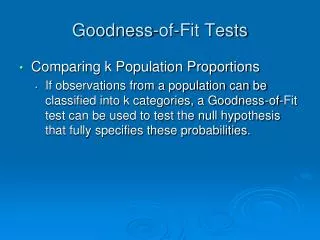
Goodness of fit testing for point processes with application to ETAS models, spatial clustering, and focal mechanisms. Frederic Paik Schoenberg, Ka Wong, and Robert Clements Point process models and ETAS Pixel-based methods Numerical summaries Error diagrams

E N D
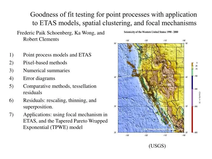
Goodness of fit testing for point processes with application to ETAS models, spatial clustering, and focal mechanisms Frederic Paik Schoenberg, Ka Wong, and Robert Clements Point process models and ETAS Pixel-based methods Numerical summaries Error diagrams Comparative methods, tessellation residuals Residuals: rescaling, thinning, and superposition. Applications: using focal mechanism in ETAS, and the Tapered Pareto Wrapped Exponential (TPWE) model (USGS)
Some point process models in seismology. Point process: random (-finite) collection of points in some space, S. N(A) = # of points in the set A. S = [0, T] x X. Simple: No two points at the same time (with probability one). Conditional intensity: (t,x) = limt,x -> 0 E{N([t, t+t) x Bx,x) | Ht} / [tx]. Ht = history of N for all times before t, Bx,x = ball around x of size x. * A simple point process is uniquely characterized by (t,x). (Fishman & Snyder 1976) Poisson process:(t,x) doesn’t depend on Ht. N(A1), N(A2), … , N(Ak) are independent for disjoint Ai, and each Poisson. Stationary (homogeneous) Poisson process: (t,x) =
Some point process models of clustering: • Neyman-Scott process: clusters of points whose centers are formed from a stationary Poisson process. Typically each cluster consists of a fixed integer k of points which are placed uniformly and independently within a ball of radius r around each cluster’s center. • Cox-Matern process: cluster sizes are random: independent and identically distributed Poisson random variables. • Thomas process: cluster sizes are Poisson, and the points in each cluster are distributed independently and isotropically according to a Gaussian distribution. • Hawkes process: parents are formed from a stationary Poisson process, and each produces a cluster of offspring points, and each of them produces a cluster of further offspring points, etc. • (t, x) = + ∑ g(t-ti, ||x-xi||). • ti < t
Aftershock activity typically follows the modified Omori law (Utsu 1971): • g(t) = K/(t+c)p.
ETAS (Epidemic-Type Aftershock Sequence, Ogata 1988, 1998): • (t, x) = (x) + ∑ g(t - ti, ||x - xi||, mi), • ti < t • where g(t, x, m) could be, for instance, K exp{m} • (t+c)p (x2 + d)q
2. Pixel-based methods.Compare N(Ai) with ∫A(t, x) dt dx, on pixels Ai. (Baddeley, Turner, Møller, Hazelton, 2005)Problems:* If pixels are large, lose power.* If pixels are small, residuals are mostly ~ 0,1.* Smoothing reveals only gross features.
Pearson residuals: Normalized difference between observed and expected numbers of events within each space-time pixel. (Baddeley et al. 2005)
3. Numerical summaries.a) Likelihood statistics (LR, AIC, BIC). Log-likelihood = ∑ log(ti,xi) - ∫ (t,x) dt dx.b) Second-order statistics. * K-function, L-function (Ripley, 1977) * Weighted K-function (Baddeley, Møller and Waagepetersen 2002, Veen and Schoenberg 2005) * Other weighted 2nd-order statistics: R/S statistic, correlation integral, fractal dimension (Adelfio and Schoenberg, 2009)
Model Assessment using Weighted K-function Usual K-function: K(h) ~ ∑∑i≠j I(|xi - xj| ≤ h), (Ripley 1979) Weight each pair of points according to the estimated intensity at the points: Kw(h)^~ ∑∑i≠j wi wj I(|xi - xj| ≤ h), (Baddeley et al. 2002) where wi = (ti , xi)-1. Asympt. normal, under certain regularity conditions. (Veen and Schoenberg 2005)
3. Numerical summaries.a) Likelihood statistics (LR, AIC, BIC). Log-likelihood = ∑ log(ti,xi) - ∫ (t,x) dt dx.b) Second-order statistics. * K-function, L-function (Ripley, 1977) * Weighted K-function (Baddeley, Møller and Waagepetersen 2002, Veen and Schoenberg 2005) * Other weighted 2nd-order statistics: R/S statistic, correlation integral, fractal dimension (Adelfio and Schoenberg, 2009) c) Other test statistics (mostly vs. stationary Poisson). TTT, Khamaladze (Andersen et al. 1993) Cramèr-von Mises, K-S test (Heinrich 1991) Higher moment and spectral tests (Davies 1977) Problems: -- Overly simplistic. -- Stationary Poisson not a good null hypothesis (Stark 1997)
4. Error DiagramsPlot (normalized) number of alarms vs. (normalized) number of false negatives (failures to predict). (Molchan 1990; Molchan 1997; Zaliapin & Molchan 2004; Kagan 2009).Similar to ROC curves (Swets 1973).Problems: -- Must focus near axes. [consider relative to given model (Kagan 2009)] -- Does not suggest where model fits poorly.
5. Comparative methods, tessellation. -- Can consider difference (for competing models)between residuals over each pixel. Problem: Hard to interpret. If difference = 3, is this because model A overestimated by 3? Or because model B underestimated by 3? Or because model A overestimated by 1 and model B underestimated by 2? Also, when aggregating over pixels, it is possible that a model will predict the correct number of earthquakes, but at the wrong locations and times. -- Better: consider difference between log-likelihoods, in each pixel. (Wong & Schoenberg 2010). Problem: pixel choice is arbitrary, and unequal # of pts per pixel…..
Problem: pixel choice is arbitrary, and unequal # of pts per pixel….. -- Alternative: use the Voronoi tessellation of the points as cells. Cell i = {All locations closer to point (xi,yi) than to any other point (xj,yj) }. Now 1 point per cell. If is locally constant, then cell area ~ Gamma (Hinde and Miles 1980)
6. Residuals: rescaling, thinning, superposing Rescaling. (Meyer 1971;Berman 1984; Merzbach &Nualart 1986; Ogata 1988; Nair 1990; Schoenberg 1999; Vere-Jones and Schoenberg 2004): Suppose N is simple. Rescale one coordinate: move each point {ti, xi} to {ti , ∫oxi(ti,x) dx} [or to {∫oti(t,xi) dt), xi }]. Then the resulting process is stationary Poisson. Problems: * Irregular boundary, plotting. * Points in transformed space hard to interpret. * For highly clustered processes: boundary effects, loss of power.
Thinning. (Westcott 1976):Suppose N is simple, stationary, & ergodic.
Thinning: Suppose inf (ti ,xi) = b. Keep each point (ti ,xi) with probability b / (ti ,xi) . Can repeat many times --> many stationary Poisson processes (but not quite independent!)
Superposition. (Palm 1943): Suppose N is simple & stationary. Then Mk --> stationary Poisson.
Superposition: Suppose sup (t, x) = c. Superpose N with a simulated Poisson process of rate c - (t, x) . As with thinning, can repeat many times to generate many (non-independent) stationary Poisson processes. Problems with thinning and superposition: Thinning: Low power. If b = inf (ti ,xi) is small, will end up with very few points. Superposition: Low power if c = sup (ti ,xi) is large: most of the residual points will be simulated.
Motivation: • Earthquakes occur primarily along faults. Aftershocks are thought to lie elliptically around previous mainshocks. • Most current models such as ETAS, which are used to produce earthquake forecasts, do not take earthquake orientation into account. • One may hope to improve existing models for earthquake forecasting by incorporating the orientations of previous earthquakes. (Kagan 1998)
Main purpose: improved forecasts. • Other purposes of ETAS • * Baseline model for • comparisons (Ogata and Zhuang 2006) • * Comparing different zones • or catalogs (Kagan et al. 2009) • * Testing hypotheses about static or • dynamic triggering (Hainzl and Ogata 2005) • * Declustering (Zhuang et al. 2002) • * Detecting anomolous seismic behavior • (Ogata 2007) 1906 SF earthquake damage (USGS)
ETAS: no use of focal mechanisms. Focal mechanisms summarize the principal direction of motion in an earthquake, as well as resulting stress changes and tension/pressure axes.
In ETAS (Ogata 1998), (t,x,m) = f(m)[(x) + ∑i g(t-ti, x-xi, mi)], where f(m) is exponential, (x) is estimated by kernel smoothing, and i.e. the spatial triggering component, in polar coordinates, has the form: g(r, ) = (r2 + d)q . Looking at inter-event distances in Southern California, as a function of the direction i of the principal axis of the prior event, suggests: g(r, ; i) = g1(r) g2( - i | r), where g1 is the tapered Pareto distribution, and g2 is the wrapped exponential.
It is well known that aftershocks occur primarily near the fault plane of their associated mainshocks (William and Frohlich 1987, Michael 1989, Kagan 1992). • One way to model anisotropic clustering is to • * identify clusters • * fit a skewed bivariate normal distribution • to aftershock locations • Problems: • Cluster identification is difficult and often subjective. • Useless for real-time hazard estimation. • Bivariate normal does not fit well.
Instead, one may incorporate focal mechanisms in ETAS by letting the triggering function g depend on the angle relative to the estimated fault plane of the previous earthquake.
Distance to next event, in relation to nodal plane of prior event (So. CA strikeslips, 1999-2007, M≥3.0, quality A or B, SCEDC).
TPWE MODEL In ordinary ETAS (Ogata 1998), l(t,x,m) = f(m)[m(x) + ∑i g(t-ti, x-xi, mi)], where f(m) is the magnitude density (e.g. Gutenberg-Richter) m(x) is estimated by kernel smoothing, and i.e. the spatial triggering component, in polar coordinates, has the form: g(r, f) = (r2 + d)-q . Looking at inter-event distances in Southern California and relative angles fi from the principal axis of the prior event suggests: g(r, f) = g1(r) g2(q - qi | r), where g1 is the tapered Pareto distribution, and g2 is the wrapped exponential.
tapered Pareto / wrapped exp. biv. normal (Ogata 1998) Cauchy/ ellipsoidal (Kagan 1996)
Model Assessment: Akaike Information Criterion (AIC): = -2 log(likelihood) + 2p. [Lower is better. Approx. c2 distributed is larger model is correct, so difference of 2 is stat. sig.] • Big (> 300 point) difference due to using the wrapped exponential • for angular separations instead of uniform distribution. • Also > 300 point difference due to tapered Pareto distribution of • distances instead of Pareto.
Cauchy/ellipse Normal TPWE TPWE vastly outperforms the normal model. Normal underpredicts density near origin (i.e. mainshock)
Thinned residuals: Data tapered Pareto / wrapped exp. Cauchy/ ellipsoidal (Kagan 1996) biv. normal (Ogata 1998)
Tapered pareto / wrapped exp. Cauchy / ellipsoidal