11.2 Goodness of Fit

1. 11.2 Goodness of Fit . .

2. Key Concept In this section we consider sample data consisting of observed frequency counts arranged in a single row or column (called a one-way frequency table). We will use a hypothesis test for the claim that the observed frequency counts agree with some claimed distribution, so that there is a good fit of the observed data with the claimed distribution. . .

3. Objectives In this section we will discussed: • Goodness-of-Fit • Equal Expected Frequencies • Unequal Expected Frequencies • Test the hypothesis that an observed frequency distribution fits (or conforms to) some claimed distribution. .

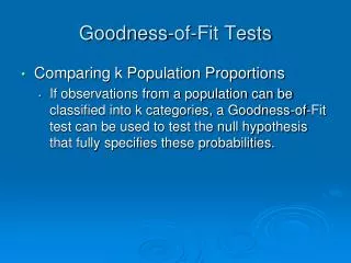
4. Definition A goodness-of-fit test is used to test the hypothesis that an observed frequency distribution fits (or conforms to) some claimed distribution. . .

5. O represents the observed frequency of an outcome. E represents the expected frequency of an outcome. krepresents the number of different categories or outcomes. nrepresents the total number of trials. Goodness-of-FitTest Notation . .

6. Goodness-of-Fit Test The data have been randomly selected. The sample data consist of frequency counts for each of the different categories. For each category, the expected frequency is at least 5. (The expected frequency for a category is the frequency that would occur if the data actually have the distribution that is being claimed. There is no requirement that the observed frequency for each category must be at least 5.) Requirements . .

7. Goodness-of-Fit Test Statistic 2=  (O – E)2 E . .

8. Goodness-of-Fit Critical Values 1. Found in Table A- 4 using k – 1 degrees of freedom, where k = number of categories. 2. Goodness-of-fit hypothesis tests are always right-tailed. . .

9. Goodness-of-Fit P-Values P-values are typically provided by computer software, or a range of P-values can be found from Table A-4. . .

10. Expected Frequencies If all expected frequencies are equal: the sum of all observed frequencies divided by the number of categories n E = k . .

11. If expected frequencies arenot all equal: Each expected frequency is found by multiplying the sum of all observed frequencies by the probability for the category. Expected Frequencies Ej = npj . .

12. A largedisagreement between observed and expected values will lead to a large value of 2 and a small P-value. A significantlylarge value of 2 will cause a rejection of the null hypothesis of no difference between the observed and the expected. Goodness-of-Fit Test • A close agreement between observed and expected values will lead to a small value of 2 and a large P-value. . .

13. Goodness-of-Fit Test “If the P is low, the null must go.” (If the P-value is small, reject the null hypothesis that the distribution is as claimed.) . .

14. Example: Data Set 1 in Appendix B includes weights from 40 randomly selected adult males and 40 randomly selected adult females. Those weights were obtained as part of the National Health Examination Survey. When obtaining weights of subjects, it is extremely important to actually weigh individuals instead of asking them to report their weights. By analyzing the last digits of weights, researchers can verify that weights were obtained through actual measurements instead of being reported. . .

15. Example: When people report weights, they typically round to a whole number, so reported weights tend to have many last digits consisting of 0. In contrast, if people are actually weighed with a scale having precision to the nearest 0.1 pound, the weights tend to have last digits that are uniformly distributed, with 0, 1, 2, … , 9 all occurring with roughly the same frequencies. Table 11-2 shows the frequency distribution of the last digits from 80 weights listed in Data Set 1 in Appendix B. . .

16. Example: (For example, the weight of 201.5 lb has a last digit of 5, and this is one of the data values included in Table 11-2.) Test the claim that the sample is from a population of weights in which the last digits do not occur with the same frequency. Based on the results, what can we conclude about the procedure used to obtain the weights? . .

17. Example: . .

18. Example: . .

19. Example: Requirements are satisfied: randomly selected subjects, frequency counts, expected frequency is 8 (> 5) Step 1: at least one of the probabilities p0, p1,… p9, is different from the others Step 2: at least one of the probabilities are the same: p0 = p1 = p2 = p3 = p4 = p5 = p6 = p7 = p8 = p9 Step 3: null hypothesis contains equality H0: p0 = p1 = p2 = p3 = p4 = p5 = p6 = p7 = p8 = p9 H1: At least one probability is different . .

20. Example: Step 4: no significance specified, use  = 0.05 Step 5: testing whether a uniform distribution so use goodness-of-fit test: 2 Step 6: see the next slide for the computation of the 2 test statistic. The test statistic 2 = 11.250, using  = 0.05 and k – 1 = 9 degrees of freedom, the critical value is 2 = 16.919 . .

21. Example: . .

22. Example: Step 7: Because the test statistic does not fall in the critical region, there is not sufficient evidence to reject the null hypothesis. . .

23. Example: Step 8: There is not sufficient evidence to support the claim that the last digits do not occur with the same relative frequency. This goodness-of-fit test suggests that the last digits provide a reasonably good fit with the claimed distribution of equally likely frequencies. Instead of asking the subjects how much they weigh, it appears that their weights were actually measured as they should have been. . .

24. Your Turn 1) .

25. H0: p1 = p2 = p3 = p4 H1: At least one of the probabilities distribution is different from the others. Input: ¼, ¼ , ¼, ¼ into L1  Expected Proportions Input: 61, 17 , 10, 12 into L2  Observed Values Go to L3: press  select “SUM(” then type “L2) * L1” and hit key MATH 2nd STAT ENTER L3  Expected Values TEST press  select “2 GOF-Test”, align L2  Observed, L3  Expected, choose the df = 4 – 1 = 3 STAT .

26. 2 = 70.16 • P-Value = 3.9445E -15 < 0.05 Reject H0 There is sufficient evidence to warrant rejection of the claim that the proportions of four categories are equally likely distributed. The result appear to support the expectation that the frequency of the first category is disproportionately high. .

27. Your Turn 2) .

28. H0: p1 = p2 = p3 = p4 = p5 = p6 = p7 H1: At least one of the probabilities distribution is different from the others. Input: 1/7, 1/7, 1/7, 1/7, 1/7, 1/7, 1/7 into L1  Expected Porportions Input: 77, 110 , 124, 122, 120, 123, 97 into L2  Observed Values Go to L3: press  select “SUM(” then type “L2) * L1” and hit key MATH 2nd STAT ENTER L3  Expected Values TEST press  select “2 GOF-Test”, align L2  Observed, L3  Expected, choose the df = 7 – 1 = 6 STAT

29. 2 = 16.8952 • P-Value = 0.0097 < 0.01 Reject H0 There is sufficient evidence to warrant rejection of the claim that the births occur on the different days with equal frequency. The result appear to support that the frequencies of the birth in weekdays are disproportionately high. .

30. .

31. .

32. Example .

33. H0: p1 = 0.301, p2 = 0.176, p3 = 0.125, p4 =0.097, p5 = 0.079, p6 = 0.067, p7 =0.058, p8 = 0.051, p9 = 0.046 H1: At least one of the proportions is not equal to the given claimed value. Input: 0.301, 0.176, 0.125, 0.097, 0.079, 0.067, 0.058, 0.051, 0.046 into L1  Expected Proportions Input: 0, 15, 0, 76, 479, 183, 8, 23, 0 into L2  Observed Values Go to L3: press  select “SUM(” then type “L2) * L1” and hit key (this calculate the Ej = npj) MATH 2nd STAT ENTER L3  Expected Values TEST press  select “2 GOF-Test, align L2  Observed, L3  Expected, choose the df = 9 – 1 = 8 STAT .

34. 2 = 3650.2514 • P-Value = 0 Reject H0 There is sufficient evidence to warrant rejection of the claim that the leading digits are from a population with a distribution that conforms to Benford’s law. It does appear that the checks are the result of fraud. .

35. Your Turn 3) .

36. H0: p1 = 9/16, p2 = 3/16, p3 = 3/16, p4 =1/16 H1: At least one of the proportions is not equal to the given claimed value. Input: 9/16, 3/16, 3/16, 1/16 into L2  Expected Proportions Input: 59, 15, 2, 4 into L2  Observed Values Go to L3: press  select “SUM(” then type “L2) * L1” and hit key (this calculate the Ej = npj) MATH 2nd STAT ENTER L3  Expected Values TEST press  select “2 GOF-Test, align L2  Observed, L3  Expected, choose the df = 4 – 1 = 3 STAT .

37. 2 = 15.8222 • P-Value = 0.0012 < 0.05 Reject H0 There is sufficient evidence to warrant rejection of the claim that the observed frequencies agree with the proportions that were expected according to principles of genetics. .

38. Recap In this section we have discussed: • Goodness-of-Fit • Equal Expected Frequencies • Unequal Expected Frequencies • Test the hypothesis that an observed frequency distribution fits (or conforms to) some claimed distribution. . .