Download
1 / 43
430 likes | 445 Views
Objective assessment of the skill of cloud forecasts: Towards an NWP- testbed. Robin Hogan, Ewan O’Connor, Andrew Barrett University of Reading, UK Maureen Dunn, Karen Johnson Brookhaven National Laboratory. Overview.

E N D
Objective assessment of the skill of cloud forecasts: Towards an NWP-testbed Robin Hogan, Ewan O’Connor, Andrew Barrett University of Reading, UK Maureen Dunn, Karen Johnson Brookhaven National Laboratory
Overview • Cloud schemes in NWP models are basically the same as in climate models, but easier to evaluate using ARM because: • NWP models are trying to simulate the actual weather observed • They are run every day • In Europe at least, NWP modelers are more interested in comparisons with ARM-like data than climate modelers (not true in US?) • But can we use these comparisons to improve the physics? • Can compare different models which have different parameterizations • But each model uses different data assimilation system • Cleaner test if the setup is identical except one aspect of physics • SCM-testbed is the crucial addition to the NWP-testbed • How do we set such a system up? • Start by interfacing Cloudnet processing with ARM products • Metrics: test both bias and skill (can only test bias of climate model) • Diurnal compositing to evaluate boundary-layer physics
Level 1b • Minimum instrument requirements at each site • Cloud radar, lidar, microwave radiometer, rain gauge, model or sondes • Radar • Lidar
Level 1c • Instrument Synergy product • Example of target classification and data quality fields: Ice Liquid Rain Aerosol
Level 2a/2b • Cloud products on (L2a) observational and (L2b) model grid • Water content and cloud fraction L2a IWC on radar/lidar grid L2b Cloud fraction on model grid
Cloud fraction Chilbolton Observations Met Office Mesoscale Model ECMWF Global Model Meteo-France ARPEGE Model KNMI RACMO Model Swedish RCA model
Cloud fraction in 7 models • All models except DWD underestimate mid-level cloud • Some have separate “radiatively inactive” snow (ECMWF, DWD); Met Office has combined ice and snow but still underestimates cloud fraction • Wide range of low cloud amounts in models • Not enough overcast boxes, particularly in Met Office model • Mean & PDF for 2004 for Chilbolton, Paris and Cabauw 0-7 km Illingworth et al. (BAMS 2007)
ARM-Cloudnet interface • First step: interface ARM products to Cloudnet processing • Now done at Reading: need to implement at Brookhaven • Is this a long-term solution? • Extra products and verification metrics still desirable
Skill and bias • If directly evaluating a climate model, can only evaluate bias • Zero bias can often be because of compensating errors • In NWP- and SCM-testbed, can also measure skill • Answers the question: was cloud forecast at the right time? • This checks whether the cloud responds to the correct forcing • Easiest to do for binary events, e.g. threshold exceedence • Metrics of skill should be: • Equitability (random and constant forecasts score zero) • Robust for rare events (many scores tend to 0 or 1) • A metric with good properties is the Symmetric Extreme Dependency Score (SEDS) – Hogan et al. (2009): • Awards score of 1 to perfect forecast and 0 for random • We have tested 3 models over SCP in 2004... • Apply with cloud-fraction threshold of 0.1
Southern Great Plains 2004 ECMWF NCEP UK Met Office (Hadley Centre Met Office)
Maureen Dunn Microbase IWC vs. ECMWF
Different mixing schemes Local mixing scheme (e.g. Meteo France) Longwave cooling • Define Richardson Number: • Eddy diffusivity is a function of Ri and is usually zero for Ri>0.25 Height (z) dqv/dz<0 Virtual potential temp. (qv) Eddy diffusivity (Km) (strength of the mixing) • Local schemes known to produce boundary layers that are too shallow, moist and cold, because they don’t entrain enough dry, warm air from above (Beljaars and Betts 1992)
Different mixing schemes Non-local mixing scheme (e.g. Met Office, ECMWF, RACMO) • Use a “test parcel” to locate the unstable regions of the atmosphere • Eddy diffusivity is positive over this region with a strength determined by the cloud-top cooling rate (Lock 1998) Longwave cooling Height (z) Virtual potential temp. (qv) Eddy diffusivity (Km) (strength of the mixing) • Entrainment velocity we is the rate of conversion of free-troposphere air to boundary-layer air, and is parameterized explicitly
Diurnal cycle composite of clouds Barrett, Hogan & O’Connor (GRL 2009) Radar and lidar provide cloud boundaries and cloud properties above site Meteo-France: Local mixing scheme: too little entrainment SMHI: Prognostic TKE scheme: no diurnal evolution Most models have a non-local mixing scheme in unstable conditions and an explicit formulation for entrainment at cloud top: good performance over the diurnal cycle
Summary and future work • One year’s evaluation over SGP • All models underestimate mid- and low-level cloud • Skill may be robustly quantified using SEDS: less skill in summer • Infrastructure to interface ARM and Cloudnet data has been tested on 1 year of data with cloud fraction and IWC • So far Met Office, NCEP, ECMWF and Meteo-France can be processed • Next implement code at BNL, with other ARM products and models • Then run on many years of ARM data from multiple sites • Question: have cloud forecasts improved in 10 years? • Next apply to SCM-testbed • Comparisons already demonstrate strong difference in performance of different boundary-layer parameterizations: non-local mixing with explicit entrainment is clearly best • We have the tools to quantify objectively improvements in both bias and skill with changed parameterizations in SCMs • Other metrics of performance or compositing methods required? • Could also forward-model the observations and evaluate in obs space?
Raw (1 hr) resolution 1 year from Murgtal DWD COSMO model Joint PDFs of cloud fraction b a d c • 6-hr averaging …or use a simple contingency table
Contingency tables Model cloud Model clear-sky Observed cloud Observed clear-sky For given set of observed events, only 2 degrees of freedom in all possible forecasts (e.g. a & b), because 2 quantities fixed: - Number of events that occurred n =a +b +c +d - Base rate (observed frequency of occurrence) p =(a +c)/n
Skill-Bias diagrams Reality (n=16, p=1/4) Forecast Under-prediction No bias Over-prediction Best possible forecast - Positive skill Random forecast Negative skill Random unbiased forecast Constant forecast of occurrence Constant forecast of non-occurrence Worst possible forecast
5 desirable properties of verification measures • “Equitable”: all random forecasts receive expected score zero • Constant forecasts of occurrence or non-occurrence also score zero • Note that forecasting the right cloud climatology versus height but with no other skill should also score zero • Difficult to “hedge” • Some measures reward under- or over-prediction • Useful for rare events • Almost all measures are “degenerate” in that they asymptote to 0 or 1 for vanishingly rare events • Dependence on full joint PDF, not just 2x2 contingency table • Difference between cloud fraction of 0.9 and 1 is as important for radiation as a difference between 0 and 0.1 • Difficult to achieve with other desirable properties: won’t be studied much today... • “Linear”: so that can fit an inverse exponential for half-life • Some measures (e.g. Odds Ratio Skill Score) are very non-linear
Hedging“Issuing a forecast that differs from your true belief in order to improve your score” (e.g. Jolliffe 2008) • Hit rate H=a/(a+c) • Fraction of events correctly forecast • Easily hedged by randomly changing some forecasts of non-occurrence to occurrence H=0.5 H=0.75 H=1
Equitability Defined by Gandin and Murphy (1992): • Requirement 1: An equitable verification measure awards all random forecasting systems, including those that always forecast the same value, the same expected score • Inequitable measures rank some random forecasts above skillful ones • Requirement 2: An equitable verification measure S must be expressible as the linear weighted sum of the elements of the contingency table, i.e. S = (Saa +Sbb +Scc +Sdd) / n • This can safely be discarded: it is incompatible with other desirable properties, e.g. usefulness for rare events • Gandin and Murphy reported that only the Peirce Skill Score and linear transforms of it is equitable by their requirements • PSS = Hit Rate minus False Alarm Rate = a/(a+c) – b/(b+d) • What about all the other measures reported to be equitable?
Some reportedly equitable measures HSS = [x-E(x)] / [n-E(x)]; x = a+d ETS = [a-E(a)] / [a+b+c-E(a)] E(a) = (a+b)(a+c)/nis the expected value of a for an unbiased random forecasting system Simple attempts to hedge will fail for all these measures LOR = ln[ad/bc] ORSS = [ad/bc – 1] / [ad/bc + 1] Random and constant forecasts all score zero, so these measures are all equitable, right?
Skill versus cloud-fraction threshold • Consider 7 models evaluated over 3 European sites in 2003-2004 HSS LOR • LOR implies skill increases for larger cloud-fraction threshold • HSS implies skill decreases significantly for larger cloud-fraction threshold
Extreme dependency score • Stephenson et al. (2008) explained this behavior: • Almost all scores have a meaningless limit as “base rate” p 0 • HSS tends to zero and LOR tends to infinity • They proposed the Extreme Dependency Score: • where n = a + b + c + d • It can be shown that this score tends to a meaningful limit: • Rewrite in terms of hit rate H =a/(a +c) and base rate p =(a +c)/n : • Then assume a power-law dependence of H on p as p 0: • In the limit p 0 we find • This is useful because random forecasts have Hit rate converging to zero at the same rate as base rate: d=1 so EDS=0 • Perfect forecasts have constant Hit rate with base rate: d=0 so EDS=1
Symmetric extreme dependency score • EDS problems: • Easy to hedge (unless calibrated) • Not equitable • Solved by defining a symmetric version: • All the benefits of EDS, none of the drawbacks! Hogan, O’Connor and Illingworth (2009 QJRMS)
Skill versus cloud-fraction threshold SEDS HSS LOR • SEDS has much flatter behaviour for all models (except for Met Office which underestimates high cloud occurrence significantly)
Skill versus height • Most scores not reliable near the tropopause because cloud fraction tends to zero SEDS EDS LBSS • New score reveals: • Skill tends to slowly decrease at tropopause • Mid-level clouds (4-5 km) most skilfully predicted, particularly by Met Office • Boundary-layer clouds least skilfully predicted HSS LOR
A surprise? • Is mid-level cloud well forecast??? • Frequency of occurrence of these clouds is commonly too low (e.g. from Cloudnet: Illingworth et al. 2007) • Specification of cloud phase cited as a problem • Higher skill could be because large-scale ascent has largest amplitude here, so cloud response to large-scale dynamics most clear at mid levels • Higher skill for Met Office models (global and mesoscale) because they have the arguably most sophisticated microphysics, with separate liquid and ice water content (Wilson and Ballard 1999)? • Low skill for boundary-layer cloud is not a surprise! • Well known problem for forecasting (Martin et al. 2000) • Occurrence and height a subtle function of subsidence rate, stability, free-troposphere humidity, surface fluxes, entrainment rate...
Key properties for estimating ½ life • We wish to model the score S versus forecast lead time t as: • where t1/2 is forecast “half-life” • We need linearity • Some measures “saturate” at high skill end (e.g. Yule’s Q / ORSS) • Leads to misleadingly long half-life • ...and equitability • The formula above assumes that score tends to zero for very long forecasts, which will only occur if the measure is equitable
Expected values of a–d for a random forecasting system may score zero: S[E(a), E(b), E(c), E(d)] = 0 But expected score may not be zero! E[S(a,b,c,d)] = S P(a,b,c,d)S(a,b,c,d) Width of random probability distribution decreases for larger sample size n A measure is only equitable if positive and negative scores cancel Which measures are equitable? ETS & ORSS are asymmetric n = 16 n = 80
Asyptotic equitability • Consider first unbiased forecasts of events that occur with probability p = ½ • Expected value of “Equitable Threat Score” by a random forecasting system decreases below 0.01 only when n > 30 • This behaviour we term asymptotic equitability • Other measures are never equitable, e.g. Critical Success Index CSI = a/(a+b+c), also known as Threat Score
What about rarer events? • “Equitable Threat Score” still virtually equitable for n > 30 • ORSS, EDS and SEDS approach zero much more slowly with n • For events that occur 2% of the time (e.g. Finley’s tornado forecasts), need n > 25,000 before magnitude of expected score is less than 0.01 • But these measures are supposed to be useful for rare events!
Possible solutions • Ensure n is large enough that E(a) > 10 • Inequitable scores can be scaled to make them equitable: • This opens the way to a new class of non-linear equitable measures Report confidence intervals and “p-values” (the probability of a score being achieved by chance)
What is the origin of the term “ETS”? • First use of “Equitable Threat Score”: Mesinger & Black (1992) • A modification of the “Threat Score” a/(a+b+c) • They cited Gandin and Murphy’s equitability requirement that constant forecasts score zero (which ETS does) although it doesn’t satisfy requirement that non-constant random forecasts have expected score 0 • ETS now one of most widely used verification measures in meteorology • An example of rediscovery • Gilbert (1884) discussed a/(a+b+c) as a possible verification measure in the context of Finley’s (1884) tornado forecasts • Gilbert noted deficiencies of this and also proposed exactly the same formula as ETS, 108 years before! • Suggest that ETS is referred to as the Gilbert Skill Score (GSS) • Or use the Heidke Skill Score, which is unconditionally equitable and is uniquely related to ETS = HSS / (2 – HSS) Hogan, Ferro, Jolliffe and Stephenson (WAF, in press)
Properties of various measures • Truly equitable • Asymptotically equitable • Not equitable
Skill versus lead time 2007 2004 • Only possible for UK Met Office 12-km model and German DWD 7-km model • Steady decrease of skill with lead time • Both models appear to improve between 2004 and 2007 • Generally, UK model best over UK, German best over Germany • An exception is Murgtal in 2007 (Met Office model wins)
Forecast “half life” Met Office DWD 2007 2004 3.0 d • Fit an inverse-exponential: • S0 is the initial score and t1/2 is the half-life • Noticeably longer half-life fitted after 36 hours • Same thing found for Met Office rainfall forecast (Roberts 2008) • First timescale due to data assimilation and convective events • Second due to more predictable large-scale weather systems 2.7 days 2.6 days 3.2 d 3.1 days 2.9 days 4.0 days 2.7 days 3.1 d 2.9 days 2.4 days 4.3 days 2.9 days 4.3 days 2.7 days
Why is half-life less for clouds than pressure? • Different spatial scales? Convection? • Average temporally before calculating skill scores: • Absolute score and half-life increase with number of hours averaged
Statistics from AMF • Murgtal, Germany, 2007 • 140-day comparison with Met Office 12-km model • Dataset released to the COPS community • Includes German DWD model at multiple resolutions and forecast lead times
Alternative approach • How valid is it to estimate 3D cloud fraction from 2D slice? • Henderson and Pincus (2009) imply that it is reasonable, although presumably not in convective conditions • Alternative: treat cloud fraction as a probability forecast • Each time the model forecasts a particular cloud fraction, calculate the fraction of time that cloud was observed instantaneously over the site • Leads to a Reliability Diagram: Perfect No resolution No skill Jakob et al. (2004)