Download
1 / 21
250 likes | 539 Views
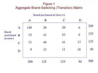
8.1 The Transition Matrix. Markov Process States Transition Matrix Stochastic Matrix Distribution Matrix Distribution Matrix for n Interpretation of the Entries of A n. Markov Process.

E N D
8.1 The Transition Matrix • Markov Process • States • Transition Matrix • Stochastic Matrix • Distribution Matrix • Distribution Matrix for n • Interpretation of the Entries of An
Markov Process • Suppose that we perform, one after the other, a sequence of experiments that have the same set of outcomes. If the probabilities of the various outcomes of the current experiment depend (at most) on the outcome of the preceding experiment, then we call the sequence a Markov process.
Example Markov Process A particular utility stock is very stable and, in the short run, the probability that it increases or decreases in price depends only on the result of the preceding day's trading. The price of the stock is observed at 4 P.M. each day and is recorded as "increased," "decreased," or "unchanged." The sequence of observations forms a Markov process.
States • The experiments of a Markov process are performed at regular time intervals and have the same set of outcomes. These outcomes are called states, and the outcome of the current experiment is referred to as the current state of the process. The states are represented as column matrices.
Transition Matrix • The transition matrix records all data about transitions from one state to the other. The form of a general transition matrix is .
Stochastic Matrix • A stochastic matrix is any square matrix that satisfies the following two properties: • 1. All entries are greater than or equal to 0; • 2. The sum of the entries in each column is 1. • All transition matrices are stochastic matrices.
Example Transition Matrix For the utility stock of the previous example, if the stock increases one day, the probability that on the next day it increases is .3, remains unchanged .2 and decreases .5. If the stock is unchanged one day, the probability that on the next day it increases is .6, remains unchanged .1, and decreases .3. If the stock decreases one day, the probability that it increases the next day is .3, is unchanged .4, decreases .3. Find the transition matrix.
Example Transition Matrix (2) The Markov process has three states: "increases," "unchanged," and "decreases." The transitions from the first state ("increases") to the other states are
Example Transition Matrix (3) The transitions from the other two states are
Example Transition Matrix (4) Putting this information into a single matrix so that each column of the matrix records the information about transitions from one particular state is the transition matrix.
Distribution Matrix • The matrix that represents a particular state is called a distribution matrix. • Whenever a Markov process applies to a group with members in r possible states, a distribution matrix for n is a column matrix whose entries give the percentages of members in each of the r states after n time periods.
Distribution Matrix for n Let A be the transition matrix for a Markov process with initial distribution matrix then the distribution matrix after n time periods is given by
Example Distribution Matrix for n Census studies from the 1960s reveal that in the US 80% of the daughters of working women also work and that 30% of daughters of nonworking women work. Assume that this trend remains unchanged from one generation to the next. If 40% of women worked in 1960, determine the percentage of working women in each of the next two generations.
Example Distribution Matrix for n (2) There are two states, "work" and "don't work." The first column of the transition matrix corresponds to transitions from "work". The probability that a daughter from this state "works" is .8 and "doesn't work" is 1 - .8 = .2. Similarly, the daughter from the "don't work" state "works" with probability .3 and "doesn't work" with probability .7.
Example Distribution Matrix for n (3) The transition matrix is . The initial distribution is
Example Distribution Matrix for n (4) In one generation, So 50% women work and 50% don't work. For the second generation, So 55% women work and 45% don't work.
Interpretation of the Entries of An The entry in the ith row and jth column of the matrix An is the probability of the transition from state j to state i after n periods.
Example Interpretation of the Entries Interpret from the last example. If a woman works, the probability that her granddaughter will work is .7 and not work is .3. If a woman does not work, the probability that her granddaughter will work is .45 and not work is .55.
Summary Section 8.1 - Part 1 • A Markov process is a sequence of experiments performed at regular time intervals involving states. As a result of each experiment, transitions between states occur with probabilities given by a matrix called the transition matrix. The ijth entry in the transition matrix is the conditional probability Pr(moving to state i|in state j).
Summary Section 8.1 - Part 2 • A stochastic matrix is a square matrix for which every entry is greater than or equal to 0 and the sum of the entries in each column is 1. Every transition matrix is a stochastic matrix. • The nth distribution matrix gives the percentage of members in each state after n time periods.
Summary Section 8.1 - Part 3 • An is obtained by multiplying together n copies of A. Its ijth entry is the conditional probability Pr(moving to state i after n time periods | in state j). Also, An times the initial distribution matrix gives the nth distribution matrix.