Download
1 / 23
250 likes | 302 Views
Fault Tree Analysis. Part 11 – Markov Model. State Space Method. Example: parallel structure of two components

E N D
Fault Tree Analysis Part 11 – Markov Model
State Space Method • Example: parallel structure of two components • Possible System States: 0 (both components in failed state); 1 (component 1 functioning, component 2 in failed state); 2 (component 2 functioning, component 1 in failed state); 3 (both components functioning).
State Space Diagram 3 2 1 0
Markov Processes • The event means that the system at time t is in state j and j = 1, 2, …,r. • The probability of this event is denoted by • The transitions between the states may be described by a stochastic process • A stochastic process satisfying the Markov property is called the Markov process.
Markov Property Given that a system is in state i at time t, i.e. X(t)=i, the future states X(t+v) do not depends on the previous states X(u), u<t. For all possible x(u) and 0≦u<t.
Stationary Transition Probability A Markov process with stationary transition properties is often called a process with no memory.
Properties of Transition Probabilities Chapman-Kolmogorov equation
Derivation of State Equation (1) • From Chapman-Kolmogorov equation • Substitute
Derivation of State Equation (2) After dividing by Δt, letting Δt→0, we get the state equations.
Simplified State Equations Since the initial state is known, the state equations can be simplified by omitting the first index i
State Equations in Matrix Notation Let Then where
Additional Properties • Notice that the sums of the columns of the transition rate matrix add up to zero. The following constraint must be imposed • The mean staying time in state j
Example • Consider a single component with two states: 1 (the component is working) and 0 (the component is in a failed state). Thus, • The state equations:
Example Since It can be derived that
Frequency of Departure from State j to State k The unconditional probability of a departure from state j to state k in the time interval (t, t+Δt] is The frequency of departure
Frequency of Departure from State j at Steady State At steady state The total frequency
Frequency of Arrival to State j at Steady State The frequency of arrival from state k to state j at the steady state The total frequency of arrivals to state j (from state equations at steady state)
Visit Frequency The visit frequency to state j is defined as the expected number of visits to state j per unit time.
Mean Duration of a Visit The total departure rate from state j Since the departure rate is constant, the duration of a stay in state j should be exponentially distributed with parameter Thus, the mean duration of stay is
A Useful Relation The mean proportion of time the system is spending in state j ( ) A special case is the formula for unavailability under corrective maintenance policy
System Availability Let S={1, 2, …, r} be the set of all possible states of a system. LetB denote the subset of states in which the system is functioning. Let F=S-B denote the states in which the system is failed. Then, the average (or long-term) system availability and unavailability are