Download
1 / 6
190 likes | 745 Views
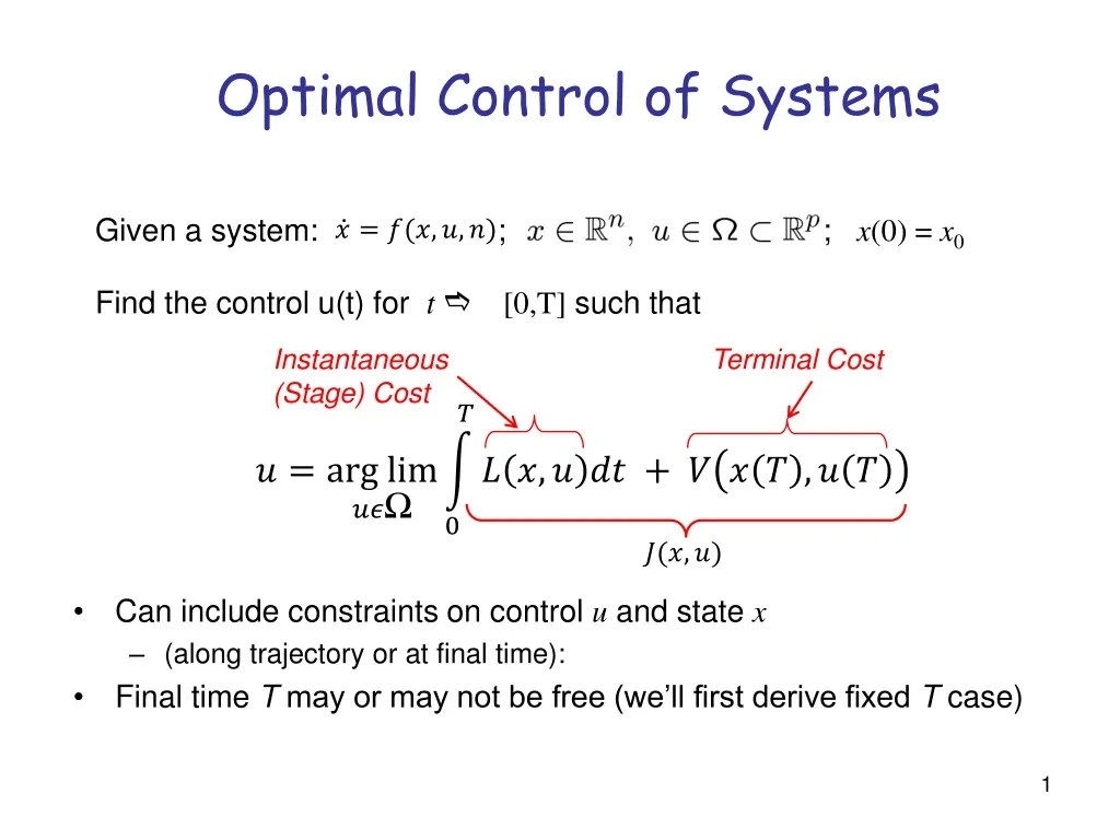
Optimal Control of Systems. Given a system: ; ; ; x (0) = x 0. Find the control u(t) for t e [0,T] such that. Instantaneous (Stage) Cost. Terminal Cost. Can include constraints on control u and state x

E N D
Optimal Control of Systems Given a system: ; ; ; x(0) = x0 Find the control u(t) for t e [0,T] such that Instantaneous (Stage) Cost Terminal Cost • Can include constraints on control uand state x • (along trajectory or at final time): • Final time T may or may not be free (we’ll first derive fixed T case)
Solution approach • Add Lagrange multiplier (t) for dynamic constraint • And additional multipliers for terminal constraints or state constraints • Form augmented cost functional: • where the Hamiltonian is: • Necessary condition for optimality: vanishes for any perturbation (variation) in x, u, or about optimum: “variations” x(t) = x*(t) + dx(t); u(t) = u*(t) + du(t); l(t) = l*(t) + dl (t); Variations must satisfy path end conditions!
Pontryagin’s Maximum Principle • Optimal (x*,u*) satisfy: • Can be more general and include terminal constraints • Follows directly from: Optimal control is solution to O.D.E. Unbounded controls 0 0 0 0
Interpretation of • Two-point boundary value problem: is solved backwards in time • is the “co-state” (or “adjoint” variable) • Recall that H = L(x,u) + Tf(x,u) • If L=0, (t) is the sensitivity of the cost to a perturbation in state x(t) • In the integral as • Recall J = … +(0)x(0)
Terminal Constraints • Assume q terminal constraints of the form: (x(T))=0 • Then • (T) = (x(T)) • Where n is a set of undetermined Lagrange Multipliers • Under some conditions, n is free, and therefore (T) is free as well • When the final time T is free (i.e., it is not predetermined), then the cost function J must be stationary with respect to perturbations T: T* + dT.In this case: • H(T) = 0
Example: Bang-Bang Control “minimum time control” H lT B>0 u +1 -1 Since H is linear w.r.t. u, minimization occurs at boundary