Operational Use of the Rapid Update Cycle

1. Stan Benjamin – mgmt, anx, model John Brown – model physics Kevin Brundage – web,NCEP Georg Grell – model Dongsoo Kim – sat data in anx Barry Schwartz – verif, obs Tanya Smirnova – model, land-sfc Tracy Smith – verif, obs Geoff Manikin – NCEP/EMC Stan Benjamin - NOAA/FSL benjamin@fsl.noaa.gov http://maps.fsl.noaa.gov - RUC/MAPS web page Operational Use of the Rapid Update Cycle COMET NWP Symposium 30 March 2000

2. The 1-h Version of the RUC Data cutoff - +20 min, 2nd run at +55 min at 0000, 1200 UTC

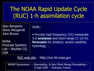
3. RUC/MAPS Purpose • Provide high-frequency mesoscale analyses and short-range numerical forecasts for users including: • aviation • severe weather forecasting • general public forecasting • other transportation • agriculture

4. RUC vector (m/s) forecast error – 0000 UTC 27 Jan 98 – 250 hPa 9h init 15z 12h init 12z 6h init 18z 3h init 21z

5. What Runs Where • Rapid Update Cycle (RUC) • Operational Version at NCEP • Mesoscale Analysis and Prediction System (MAPS) • Experimental Version at NOAA/ERL/FSL • Backup RUC • Advanced, hardened version running at FSL • Used after NCEP fire (1 Oct – 15 Nov), during NCEP outages since then (Essentially the same software. New capabilities tested first in MAPS at FSL)

6. Uses of the RUC • Explicit Use of Short-Range Forecasts • Monitoring Current Conditions with Hourly Analyses • Evaluating Trends of Longer-Range Models Some places where the RUC is used • Aviation Weather Center - airmets, sigmets • Storm Prediction Center - severe weather watches • FAA – CWSUs, WARP, air traffic management (CTAS), ITWS.. • National Weather Service Forecast Offices • Airline Forecasting Offices • NASA Space Flight Centers • Private vendors • Other AWRP PDTs – icing, turbulence, AGFS/ADDS/RTVS, convective weather, winter weather

7. NWS Forecast Discussion Use of RUC - Feb 1999 – Feb 2000 200-500 100-199 40-99 20-39 10-19

8. RUC/MAPS web page - http://maps.fsl.noaa.gov

9. 40km RUC topography

10. Hourly Data for 40 km RUC-2 Data Type ~Number Freq. Use Rawinsonde (inc. special obs) 80 /12h NCEP and FSL WPDN/NPN profilers 31 / 1h NCEP and FSL - 405 MHz Boundary layer profilers 15 / 1h FSL only RASS (WPDN and PBL) 15 / 1h FSL only VAD winds (WSR-88D) 110-130 / 1h **NCEP & FSL Aircraft (ACARS)(V,temp) 700-3000 / 1h NCEP and FSL Surface - land (V,psfc,T,Td) 1500-1700 / 1h NCEP and FSL Buoy 100-200 / 1h NCEP and FSL **not used since 1/99 in RUC or EDAS pending QC issues Yellow items new for RUC-2

11. Hourly Data for 40 km MAPS/RUC-2 (cont). Data Type ~Number Freq. Use GOES precipitable water 1000-2500 / 1h NCEP and FSL GOES high-density cloud drift winds (IR, VIS, WV cloud top) 1000-2500 / 3h NCEP and FSL SSM/I precipitable water 1000-4000 /2-6h NCEP only Ship reports 10s / 3h NCEP only Reconnaissance dropwinsonde a few / variable NCEP only Yellow items new for RUC-2 Real-time observation counts at http://maps.fsl.noaa.gov for RUC-2 and 40-km MAPS

12. Advantages of q Coordinates for Data Assimilation Analysis - adaptive 3-d correlation structures and analysis increments, esp. nearbaroclinic zones, vertical spreading = f(q) - improved coherence of observations near fronts for QC Forecast Model - reduced vertical flux through coordinate surfaces, leading to reduced vertical dispersion -- much of vertical motion implicit in 2-d horiz. advection - conservation of potential vorticity - reduced spin-up problems (Johnson et al. 93 MWR)

13. RUC hybrid-b levels - cross-section Hybrid-b levels - solid q levels (every 6 K) - dashed No discontinuities at q/stransitions

14. RUC generalized vertical coordinate Cross section A Cross section B A Reference v values (220-450K) assigned to each of (40) RUC levels. More generalized levels become terrain-following levels in warmer parts of domain/times of year B 1800 UTC 24 February 2000 Surface v

15. Solution of continuity equation S = generalized vertical coordinate surfaces • Solve mass convergence 0 =0 for s= =0 0 for s=s

16. Effect of vertical coordinate on frontal features Turbulence diagnostic at FL200 (20,000 ft) - calculated from native grid from both MesoEta and RUC (matched forecast times) Sharper frontal resolution with RUC despite coarser horizontal resolution and fewer vertical levels

17. Rapid Update Cycle – Present and Next Version 1999 Operations 2000-01 Operations Resolution 40 km, 40 q/s levels 2015 km, 40  50-60 q/s levels Analysis Optimal interpolation on 3-d variational technique on generalized on generalized q/s surfaces q/s surfaces, hydrometeor analysis w/ GOES…, use raw instead of interp. obs Assimilation Intermittent 1-h cycle Intermittent 1-h cycle Stable clouds Mixed-phase cloud microphysics MM5), Improved microphysics, /precipitation explicit fcst of cloud water, rain water, addition of drizzle snow, ice, graupel, no. concentration of ice particles Sub-grid-scale Grell (1993) Modified Grell, scale dependence, precipitation shallow convection, interaction w/ cloud microphysics Turbulence Burk-Thompson explicit TKE scheme Refined Burk-Thompson or e- Radiation MM5 LW/SW scheme, f(hydrometeors) Refined MM5 scheme Land-sfc processes 6-level soil/veg model (Smirnova, 2-layer snow, improved hi-res land use, 1997, 1999) w/ frozen soil, 1-layer snow improved cold season processes Sfc conditions Daily 50km SST/14 km LST, Combine sat Tskin, use 3-d soil type 0.14 monthly NDVI veg frac, cycled soil moisture/temp, snow depth/temp

18. RUC-2 Analysis • Background (1-h fcst usually) subtracted from all obs • Analysis is of forecast error • QC - buddy check, removal of VADs w/ possible bird contamination problems • 3-part analysis (all using optimal interpolation) • 1) univariate precipitable water (PW) analysis - using satellite PW obs - update mixing ratio field • 2) z/u/v 3-d multivariate analysis • update v based on height/thickness analysis increment • update psfc from height analysis increment at sfc • update u/v at all levels • Partial geostrophic balance – vertically dependent, weakest at surface

19. RUC-2 Analysis, cont. - 3) univariate analyses • condensation pressure at all levels • v at all levels • update u/v near sfc and psfc (univariate analysis) with smaller correlation lengths • Pass through soil moisture, cloud mixing ratios, snow cover/temperature (will alter these fields in future, cloud analysis parallel cycle now running)

20. Sounding comparison – RUC grid vs. raob Raob sounding RUC2 grid sounding Close fit to observations in RUC2 analysis

21. Fix to use of sig-level data Raob RUC after fix RUC before fix 7 April 99 significant-level fix in RUC-2

22. Use of ‘minimum topography’for 2m T/Td fields from RUC2 RUC2 2m T/Td fields are not valid at model terrain surface Instead, they are derived from model surface fields and lapse rates in lowest 25 mb to estimate new values using a different topography field that more closely matches actual METAR elevations “Minimum topography” – minimum 10km value inside each 40km grid box, then updated with high-resolution analysis using actual METAR elevations.

23. RUC2 topography fields Minimum topo for 2m T/Td Model topo

24. RUCS 60 km Hourly Surface Analyses (same as AWIPS MSAS) • Draws fairly closely to data • Persistence background field (1 hr previous analysis • QC vulnerable to consistent data problems • no consistency with terrain effects except as reflected in observations • MAPS sea-level pressure, (Benjamin & Miller, 1990 MWR) • Blending to data-void region from NGM

25. Surface Analyses/Forecasts in RUC-2 • integrated with 3-d 40 km 1 hr cycle • dynamic consistency with model forecast => accounts for: • land/water, mtn circulations, sea/lake breezes, snow cover, vegetation… • improved quality control - model forecast background prevents runaway bullseyes • forecasts out to 12 hr in addition to hourly analyses

26. Divergence - 0900 UTC 20 Jan 98 (blue - conv, green/yellow - div) RUC2 Surface Analysis Topographical features more evident with model background RUCS 60km surface analysis Little consistency with nighttime drainage

27. Divergence - RUC2 Surface Analysis - 0600Z 19 April 96 Consistency with topographical features in model (land/water roughness length variations in this case)

28. RUC-2 use of surface data All winds, sfc pressure obs used T/Td used if abs (Pstation - Pmodel) < 70 mb - about 90% west of 105ºW, 99% east of 105ºW Eta48 Eta29 RUC40 FGZ 0 18 10 TUS 60 13 44 SLC 59 68 59 MFR 109 48 67 OAK 1815 25 SAN 12 5 23 DRA 42 29 34 GJT 98 105 65 RIW 104 27 16 GEG 4 11 1 GTF 26 4 14 UIL 14 9 11 SLE 50 15 22 BOI 55 21 24 GGW 29 13 5 VBG 5 32 3 |pmodel - pstn| ** within 5 mb of closest fit

29. Key issues in use of surface data in 3-d data assimilation • Goals • 1) best estimate of current conditions • 2) best subsequent 3-d model forecast • Reduction between station elevation and model terrain • Use local lapse rate for temperature • Moisture? – maintain RH (used in RUC), use hygrolapse rate? • Use consistent and reversible algorithms for • going from station to model terrain (analysis) • going from model terrain to mini-topo (post-processing) • Vertical representativeness of surface data • RUC – potential temperature separation • Horizontal representativeness of surface data • RUC – potential temperature separation in horizontal adds to “vertical distance”

30. Weaknesses in use of surface data in current RUC 3-d analysis Influence of surface data in analysis limited to lowest 6 levels (lowest 25-40 mb) How to determine depth of influence – Does an error at the surface imply the same forecast error throughout the boundary layer? Sometimes yes, sometimes no.

31. RUC-2 use of surface data All winds, sfc pressure obs used T/Td used if abs (Pstation - Pmodel) < 70 mb - about 90% west of 105ºW, 99% east of 105ºW Eta48 Eta29 RUC40 FGZ 0 18 10 TUS 60 13 44 SLC 59 68 59 MFR 109 48 67 OAK 1815 25 SAN 12 5 23 DRA 42 29 34 GJT 98 105 65 RIW 104 27 16 GEG 4 11 1 GTF 26 4 14 UIL 14 9 11 SLE 50 15 22 BOI 55 21 24 GGW 29 13 5 VBG 5 32 3 |pmodel - pstn| ** within 5 mb of closest fit

32. Key issues in use of surface data in 3-d data assimilation • Goals • 1) best estimate of current conditions • 2) best subsequent 3-d model forecast • Reduction between station elevation and model terrain • Use local lapse rate for temperature • Moisture? – maintain RH (used in RUC), use hygrolapse rate? • Use consistent and reversible algorithms for • going from station to model terrain (analysis) • going from model terrain to mini-topo (post-processing) • Vertical representativeness of surface data • RUC – potential temperature separation • Horizontal representativeness of surface data • RUC – potential temperature separation in horizontal adds to “vertical distance”

33. Weaknesses in use of surface data in current RUC 3-d analysis Influence of surface data in analysis limited to lowest 6 levels (lowest 25-40 mb) How to determine depth of influence – Does an error at the surface imply the same forecast error throughout the boundary layer? Sometimes yes, sometimes no.

34. RUC surface temperature forecasts - verification against all METARs in RUC domain Excellent analysis fit to surface obs (also wind, Td) 3-h forecast better than 3-h persistence RMS error Bias (obs - forecast) persistence Validation time Validation time

35. RUCDigital FilterInitialization 40 Dt forward 40 Dt backward - digital filter avg of model values Produces much smoother 1-h fcst Mean absolute sfc pres tendency each Dt in successive RUC runs

36. RUC-2 Model • Prognostic variables • Dynamic - (Bleck and Benjamin, 93 MWR) • v, p between levels, u, v • Moisture - (MM5 cloud microphysics) • q v, qc, qr, qi, qs, qg, Ni (no. conc. ice particles) • Turbulence - (Burk-Thompson, US Navy, 89 JAS) • Soil - temperature, moisture - 6 levels (down to 3 m) • Snow - water equivalent depth, temperature (soil/snow/veg model - Smirnova et al., 1997 MWR)

37. RUC-2 Model, cont. • Numerics • Continuity equation • flux-corrected transport (positive definite) • Advection of v, all q (moisture) variables • Smolarkiewicz (1984) positive definite scheme • Horizontal grid • Arakawa C • Vertical grid • Non-staggered, generalized vertical coordinate currently set as isentropic-sigma hybrid

38. RUC-2 Model, cont. • Cumulus parameterization • Grell (Mon.Wea.Rev., 1993) • simplified (1-cloud) version of Arakawa-Schubert • includes effects of downdrafts • Digital filter initialization (Lynch and Huang, 93 MWR) • +/- 40 min adiabatic run before each forecast

39. (Reisner, Rasmusssen, Bruintjes, 1998, QJRMS) Processes in RUC2/MM5 microphysics

40. RUC2 case study - Quebec/New England ice storm - 9 Jan 1998 500 mb height/vorticity - 9h RUC2 fcst valid 2100 UTC

41. RUC2 9h fcst - Surface temp (image), MSLP (beige isobars)

42. N-S cross-section - temperature (isopleths, int = 2 deg C, solid for > 0) RH (image), 9h RUC2 forecast YUL

43. Montreal ice storm - 9h RUC2 forecast valid 2100 9 Jan 98. N-S cross sections of RUC2 microphysics Water vapor mixing ratio / q Cloud water mixing ratio | YUL/Montreal Graupel mixing ratio Rain water mixing ratio

44. 40 km RUC versus 32 km Eta June-July 1999

45. 40 km RUC versus 32 km Eta June-July 1999

46. RUC vs. Eta 12-h fcsts250mb RMS vector error 12 11 10 9 8 7 6 5 From 80km grids for both models RUC uses 24h Eta for lateral boundary conditions Comparable skill, potential for ensembles

47. RUC 1, 3, 6, 12h forecasts valid at same time (against 0000 and 1200 UTC rawinsonde data) Better wind and temperature forecasts with use of more recent asynoptic data

48. RUC/MAPSLand-surfaceProcessParameterization (Smirnova et al. 1997, MWR; 1999, JGR) Ongoing cycle of soil moisture, soil temp, snow cover/depth/temp) 2-layer snow model

49. Previous MAPS vegetation New vegetation – BATS classes Addition of high-resolution EOS vegetation-type data to backup RUC - September 1999 NCEP RUC – summer 2000

50. RUC/MAPS cycling of soil/snow fields - soil temperature, soil moisture - snow water equivalent, snow temperature MAPS snow water equivalent depth (mm) 5 Jan 1999 1800 UTC NESDIS snow cover field 5 Jan 1999 2200 UTC 1” 2” 3” 4” 5”