Download
1 / 38
390 likes | 705 Views
Learning Causality. Some slides are from Judea Pearl’s class lecture http://bayes.cs.ucla.edu/BOOK-2K/viewgraphs.html. Rain. Mud. Other causes of mud. A causal model Example.

E N D
Learning Causality Some slides are from Judea Pearl’s class lecture http://bayes.cs.ucla.edu/BOOK-2K/viewgraphs.html
Rain Mud Other causes of mud A causal model Example • Statement ‘rain causes mud’ implies an asymmetric relationship: the rain will create mud, but the mud will not create rain. • Use ‘→’ when refer such causal relationship; • There is no arrow between ‘rain’ and ‘other causes of mud’ means that there is no direct causal relationship between them;
A E C F B D Directed (causal) Graphs • A and B are causally independent; • C, D, E, and F are causally dependent on A and B; • A and B are direct causes C; • A and B are indirect causes D, E and F; • If C is prevented from changing with A and B, then A and B will no longer cause changes in D, E and F.
Causal Structure (cont’d) • A Causal Structure serves as a blueprint for forming a “casual model” – a precise specification of how each variable is influenced by its parents in the DAG. • We assume that Nature is at liberty to impose arbitrary functional relationships between each effect and its causes and then to perturb these relationships by introducing arbitrary disturbance; • These disturbances reflect “hidden” or unmeasurable conditions.
Causal Model (Cont’d) • Once a causal model M is formed, it defines a joint probability distribution P(M) over the variables in the system; • This distribution reflects some features of the causal structure • Each variable must be independent of its grandparents, given the values of its parents • We may allowed to inspect a select subset OV of “observed” variables to ask questions about P[o], the probability distribution over the observations; • We may recover the topology D of the DAG, from features of the probability distribution P[o].
Structure Preference (Cont’d) • The set of independencies entailed by a causal structure imposes limits on its power to mimic other structure; • L1 cannot be preferred to L2 if there is even one observable dependency that is permitted by L1 and forbidden by L2; • L1 is preferred to L2 if L2 has subset of L1’s independence; • Thus, test for preference and equivalence can sometimes be reduced to test dependencies, which can be determined by topology of the DAGs without concerning parameters.
Examples • {a,b,c,d} reveal two independencies: • a is independent of b; • d is independent of {a,b} given c; • Assume further that the data reveals no other independencies; • a = having a cold; • b = having hay fever; • c = having to sneeze; • d = having to wipe one’s nose.
Arbitrary relations between a and b minimal Example (Cont’d) • {a,b,c,d} reveal two independencies: • a is independent of b; • d is independent of {a,b} given c; Not minimal: fails to impose conditional Independence between d and {a,b} Not consistent with data: impose marginal independence between d and {a,b}
Stability The stability condition states that, as we vary the parmeters from to, no indpendence in P can be destroyed. In other words, if the independency exists, it will always exists.
Stable distribution • A probability distribution Pis a faithful/stable distribution if there exist a directed acyclic graph (DAG) Dsuch that the conditional independence relationship in Pis also shown in the D, and vice versa.
IC algorithm (Inductive Causation) • IC algorithm (Pearl) • Based on variable dependencies; • Find all pairs of variables that are dependent of each other (applying standard statistical method on the database); • Eliminate (as much as possible) indirect dependencies; • Determine directions of dependencies;
Comparing abduction, deduction and induction A => B A --------- B • Deduction: major premise: All balls in the box are black minor premise: These balls are from the box conclusion: These balls are black • Abduction: rule: All balls in the box are black observation: These balls are black explanation: These balls are from the box • Induction: case: These balls are from the box observation: These balls are black hypothesized rule: All ball in the box are black A => B B ------------- Possibly A Whenever A then B but not vice versa ------------- Possibly A => B Induction: from specific cases to general rules; Abduction and deduction: both from part of a specific case to other part of the case using general rules (in different ways) Source from httpwww.csee.umbc.edu/~ypeng/F02671/lecture-notes/Ch15.ppt
IC Algorithm (Cont’d) • Input: • P – a stable distribution on a set V of variables; • Output: • A pattern H(P) compatible with P; Patten: is a partially directed DAG • some edges are directed and • some edges are undirected;
Sab a b Sab a ╨ b a b Not Sab IC Algorithm: Step 1 • For each pair of variables a and b in V, search for a set Sab such that (a╨b | Sab) holds in P – in other words, a and b should be independent in P, conditioned on Sab . • Construct an undirected graph G such that vertices a and b are connected with an edge if and only if no set Sab can be found.
Yes a a ╨ b C c a No b c b IC Algorithm: Step 2 • For each pair of nonadjacent variables a and b with a common neighbor c, check if c Sab. • If it is, then continue; • Else add arrowheads at c • i.e a→ c ← b
Other causes of mud Other causes of mud Rain Rain Mud Mud Example
IC Algorithm Step 3 • In the partially directed graph that results, orient as many of the undirected edges as possible subject to two conditions: • The orientation should not create a new v-structure; • The orientation should not create a directed cycle;
b c a b c b c Rules required to obtaining a maximally oriented pattern • R1: Orient b — c into b→c whenever there is an arrow a→b such that a and c are non adjacent;
a b a c b a b Rules required to obtaining a maximally oriented pattern • R2: Orient a — b into a→b whenever there is a chain a→c→b;
a b c a b a b d Rules required to obtaining a maximally oriented pattern R3: Orient a — b into a→b whenever there are two chains a—c→b and a—d→b such that c and d are nonadjacent;
a b a b Rules required to obtaining a maximally oriented pattern R4: Orient a — b into a→b whenever there are two chains a—c→d and c→d→b such that c and b are nonadjacent; a c d c d b
IC* Algorithm • Input: • P, a sampled distribution; • Output: • core(P), a marked pattern;
IC* Algorithm: Step 1 For each pair of variables a and b, search for a set Sab such that a and b are independent in P, conditioned on Sab. If there is no such Sab, place an undirected link between the two variables, a – b.
IC* Algorithm: Step 2 • For each pair of nonadjacent variables a and b with a common neighbor c, check if cSab • If it is, then continue; • If it is not, then add arrow heads pointing at c (i.e. a c b). • In the partially directed graph that results, add (recursively) as many arrowheads as possible, and mark as many edges as possible, according to the following two rules:
a a c c * b b IC* Algorithm: Rule 1 • R1: For each pair of non-adjacent nodes a and b with a common neighbor c, if the link between a and c has an arrow head into c and if the link between c and b has no arrowhead into c, then add an arrow head on the link between c and b pointing at b and mark that link to obtain c –* b;
IC* Algorithm: Rule 2 • R2: If a and b are adjacent and there is a directed path (composed strictly of marked links) from a to b, then add an arrowhead pointing toward b on the link between a and b;