Download

1 / 40
420 likes | 439 Views
Causality. Advanced statistical analysis of epidemiological studies Theis Lange Departement of Biostatistics Mail: thlan@sund.ku.dk. Outline for today. Introduction to the why and what of causality. A mathematical langue for causality. Tools and techniques.

E N D
Department of Biostatistics Causality Advanced statistical analysis of epidemiological studies Theis Lange Departement of Biostatistics Mail: thlan@sund.ku.dk
Department of Biostatistics Outline for today • Introduction to the why and what of causality. • A mathematical langue for causality. • Tools and techniques. • A more advanced topic: Mediation (if time permits) • 12:45-13:00: Course evaluation (Per) • 13:30 onwards: Exercise
Department of Biostatistics Why? • Why do we whish to discuss causality and not ”just” do statistics? • Here is a local example to motivate us: • SVAR:
Department of Biostatistics The moral of the local example • The same numbers can be interpreted in many ways ;-) • All in this room know that: • Association is not causation! • but do you think that the readers of - and (most) participants in - the “efterløn”-discussion remembered this? • Do you think that any of the measures mentioned in the articles capture the effect of abolishing efterløn? • So at the very least we need to think about causality because our audiences often do.
Department of Biostatistics The two sources of data • Observational studies • Big • Cheap • Denmark is the perfect place for conduction such studies. • BUT: It is difficult to interpret the result. • Randomized studies • Small • Expensive • Denmark is only a bit better than the rest of the world for conducting such studies. • BUT: It is easy to interpret the result.
Department of Biostatistics The randomized study revisited • A randomized study has two key components. • The inclusion criterions • Define who are eligible to participate in the trial. • Thereby they define to which population the obtained results apply. • In drug trails children, pregnant, and elderly are often routinely excluded even though the drug will be given to these groups as well. • The randomization • For each person enrolled in the trial, which treatment they receive is decided by “the flip of a coin”. • Probability of treatment can depend on baseline characteristics; e.g. sex or age, but the actual treatment choice is completely random.
Department of Biostatistics What is a causal effect? • Assume that you are interested in understanding the impact of a given variable (the exposure) on one or more outcomes. • If you can envies (at least in principle) a way to measure the impact of the exposure through a randomized trial this will be the causal effect of the exposure. • Thus a causal effect is: • Any effect which can (disregarding costs and ethics) be estimated from a randomized trial. • The inclusion criterions for the enviesed randomized trial define to which population the causal effect applies.
Department of Biostatistics What is causal inference? • For obvious reasons we cannot always conduct randomized trails. • Several active areas of research, collectively referred to as causal inference, aim at deducing causal effects from observational studies. • Participants from many backgrounds including: • Epidemiologists • Statisticians • Economists • Philosophers • Computer scientists • Physicists • …
Department of Biostatistics Causal inference books • The bible – old testament: • J. Pearl (2009)Causality • The bible – new testament? • M.A. Hernán & J.M. Robins (2011?)Causal InferenceAvailable online at:http://www.hsph.harvard.edu/faculty/miguel-hernan/causal-inference-book/ • Some other recent: • S. Morgan & C. Winship (2007)Counterfactuals and Causal Inference • D. Freedman (2010)Statistical Models and Causal Inference
Department of Biostatistics DAG: A key tool A Y • DAGs (Directed Acyclic Graphs) are often used to depict causal relationships. • The DAG is built from substance knowledge not from the data at hand. • The real information in a DAG is in the direction of the arrows • and in which arrows that are NOT there. • Remember also to think of unmeasured confounders/variables (U in the DAG above). • Rules for manipulating DAGs is outside today's scope. C (U)
Department of Biostatistics The langue of counterfactuals • Counterfactuals variables have been developed to provide a firm (mathematical) footing for arguments about cause and effect. • The counterfactual variable Ya denotes the value the outcome (Y) would take if exposure (A) was set to a by an intervention. • For every individual there exists many counterfactual variables corresponding to all possible levels of exposure. • Thus counterfactual variables describe what would have happened if we had intervened on exposure. • For this reason they are also referred to as potential outcomes (or more popular: “What-if-mathematics”)
Department of Biostatistics Average treatment effect • Naturally we only observe one outcome for each person so we cannot compare Ya=0 and Ya=1 directly. • We can, however, compute average causal effects: ACE = E[Ya=1 - Ya=0] = E[Ya=1] - E[Ya=0] • The average (E in the equation above) is to be interpreted as taken across the target population. • Average causal effect is therefore also called population wide effects. • ACE is the effect we would see in a randomized study of the effect of A! Note that the choice of population to take average across corresponds to the inclusion criterions of the randomized study
Department of Biostatistics Computing ACE from data • Clearly counterfactuals are only useful if they can be related to the actual observed data.We must therefore impose three assumptions: • No-unmeasured confounders of exposure-outcome relation. • Positivity: P(A=a|C=c) > 0 for all a,c.In words: In all strata of confounders there is a positive probability of both exposure=0 and exposure=1. • Consistency: Ya=A = Y, where Y denotes the observed outcome. In words: If we intervened to set the exposure to the level it would naturally have taken, we do not change the outcome.
Department of Biostatistics Computing ACE from data in practice A Y • Consider the DAG above with A, C, and Y binary. • Under the assumptions from the last slide it holds that: E[Ya=1] = E[Ya=1 | C=0]P(C=0) + E[Ya=1| C=1]P(C=1) = E[Y | C=0, A=1]P(C=0) + E[Y | C=1, A=1]P(C=1) • With more confounders or other types of variables this procedure breaks down. C
Department of Biostatistics Methods for computing casual effects • The most important tools for estimating causal effects are: • Regression • Matching • Propensity score techniques • Inverse probability of treatment weighting(Marginal structural models) • Instrumental variables • In the following we will discuss these tools in varying degree of detail based on a 2006 paper.
Department of Biostatistics Example: Kurth et al., Amer. J. Epi., 2006 • Goal: Comparison of different tools for estimating causal effects. • Data: In-hospital mortality in 6269 stroke patients treated (212) or not treated with tissue plasminogen activator (t-PA). Data from Westphalian Stroke Registry, Germany.
Department of Biostatistics Example: Kurth et al., Amer. J. Epi., 2006 • Look at distribution of pre-treatment variables (we assume these are adequate to control for confounding):
Department of Biostatistics Multiple Regression • A standard approach to account for differences between treatment groups is multiple logistic regression.In SAS:proc logistic … • Interpretation: For fixed values of all confounders t-Pa treatment is significantly associated with death; OR=1.93.
Department of Biostatistics (Simple) matching • Match each person on treatment to a person not on treatment with the same values of the confounders. • BUT we have 16 confounders so it is impossible to do this… • Let us try to be smarter!
Department of Biostatistics Propensity scores • Definition (Rosenbaum and Rubin (Biometrika, 1983)):The propensity score (e(C)) is the probability that an individual would have been treated based on that individual’s observed pre-treatment variables: e(C) = P(A = 1 | C) • Idea: In a randomized study, treatment assignment A and pre-treatment variables C are independent. • The propensity score e(C) has the property that treatment assignment A is independent of pre-treatment variables C for any given value of e(C). • That is, treated and untreated individuals with the same e(C) have identical distributions of C.
Department of Biostatistics Computing propensity score • The propensity score is unknown and must be estimated. For a binary A, logistic regression is the obvious choice for e(C). • Why should one choose a propensity score approach rather than including c in a standard regression model? • We can ask the doctor what is important when he or she decides who to treat (A | C) – we cannot ask nature what is important when “she decides” who will die (Y | C)! • If P(Y = 1) is small and P(A = 1) is not small then e(C) allows a richer model, e.g. including many interactions. • It has been argued that over-fitting when developing the model for e(C) may not be a bad thing to do.
Department of Biostatistics Computing propensity score in SAS • Use proc logistic to fit a logistic regression and save the predicted probabilities in a new dataset. • proc logistic data = stroke; • class tPa (…); • model tPa(event=‘1’) = age sex (…); • output out=psdataset pred=ps; • run;
Department of Biostatistics Using propensity scores: Matching • If there are no unmeasured confounders the causal effect of treatment can be obtained by comparing individuals from the two treatment arms with the same propensity score. • The easiest way to do this is for every person on treatment to find the person from the control group, which has the same propensity score (or very close) and match those. • In SAS: • /* Load the gmatch macro from: http://mayoresearch.mayo.edu/mayo/research/biostat/upload/gmatch.sas */ • %gmatch(data=psdataset, group=tPa, id=ptID, • mvars=ps, wts=1, dmaxk=0.05,out=mtch, • seedca=87877,seedco=987973);
Department of Biostatistics Using propensity scores: Matching in SAS • data work.ids; set work.Mtch; • ptID = __IDCA; caseID = __IDCA; output; • ptID = __IDCO; caseID = __IDCA; output; • keep ptID caseID; run; • PROC SORT DATA=ids OUT=ids2 ; • BY ptID; • RUN; • DATA matchedFinal; • MERGE psdataset ids2 (in=in2); • BY ptID; • if in2; • run;
Department of Biostatistics Using propensity scores: Matching II • In the stroke data 96% of the 212 patients who received treatment could be matched on propensity score +/- 0.05. • After matching we had this distribution of pre-treatment variables (NB: Doctors love a table like this!)
Department of Biostatistics Using propensity scores: Matching III • Finally the causal effect of treatment can be computed by analyzing a simple 2x2 table in the matched data set. • (However, this approach does not account for the dependence due to the matching. A proc genmod with a repeated statement would be better) • Interpretation: Imagine two version of the world both with pre-treatment distribution as in the treatment group; in one version all received t-Pa treatment, in the other none did. Odds ratio for death will be 1.17 between the two worlds.
Department of Biostatistics Using propensity scores: Regression • Instead of matching on the propensity score it could instead be included in a logistic regression. • The Propensity score can be included either continuous or in e.g. deciles. And you can include (in addition to tPa) only the propensity score or also a few pre-treatment variables on top. • Interpretation: Just like ordinary multiple regression(!) • My view: I cannot see why you would prefer this instead of ordinary regression.
Department of Biostatistics Inverse probability of treatment weighting • Matching on propensity scores seems promising, but on the other hand you discharge almost all of your data (6,269 vs. 406 observations)! • Inverse probability of treatment weighting (IPTW) is an attempt to fix this. • Instead of matching using propensity scores (and loose a lot of observations) we attempt to reweight the observations to mimic a randomized study.
Department of Biostatistics IPTW (continued) • For each person compute a weight as 1 divided by the probability of receiving the treatment they actually got:Weight for people on treatment = 1/e(Ci)Weight for people not on treatment = 1/(1-e(Ci)) • The average of the counterfactual Ya=1 can now be estimated as the weighted average (using the weights above) of all persons receiving treatment. • Intuition: If person whose pre-treatment variables indicate that he is unlikely to get treatment get it anyway, he should be up-weighted because in a randomized study this group would have had 50% chance of treatment.
Department of Biostatistics IPTW in SAS • Compute and save propensity scores as before. • Compute weights by: • data work.IPTWdataset; • set work.psdataset; • if tPa = 1 then w = 1/ps; • if tPa = 0 then w = 1/(1-ps); • run; • Next fit a logistic regression using these weights: • proc genmod data=work.IPTWdataset; • class tPa, ptID; • model death = tPa / error=B; • weight w; • repeated subject = ptID / type = IND; • run;
Department of Biostatistics IPTW – Result • Interpretation of IPTW measure:Imagine two version of the world both with pre-treatment variable distribution as in the general population; in one version all received t-Pa treatment, in the other none did. Odds ratio for death will be 10.77 between the two worlds.
Department of Biostatistics Result overview • All the effects highlighted in yellow are different estimates of the same parameter (why?), • but the other are estimates of different parameters.
Department of Biostatistics Explaining the difference between PS and IPTW • Could it be estimation uncertainty? • Better to look at the distribution of confounders/PS between treatment groups.
Department of Biostatistics Instrumental variables • Until now we have discussed techniques to estimate causal effects from observational studies in the absence of unmeasured confounders. • But what if we know there are important confounders, which cannot be measured (as in the DAG below)? • Is all hope lost? A Y (U)
Department of Biostatistics Instrumental variables (II) • This type of problem is often been encountered in economics and they have developed an elegant solution namely instrumental variables. • An instrument (I) is a variable which is associated with exposure (A), but only associated with the outcome through the exposure; see the DAG below: • By using the instrument we can get an unbiased estimat of the effect of exposure on outcome without knowing U!!!! I A Y (U)
Department of Biostatistics Instrumental variables - intuition • The basic idea of instrumental variables (or IV among friends) is: • To use the instrument to predict exposure for each person in the sample. • To model the relationship between the predicted exposure and the actual outcome. Thus exposure is replaced by predicted exposure and since the predicted exposure only depends on the instrument the relation between predicted exposure and outcome is unconfounded. • The art in IV is to come up with a good instrument.
Department of Biostatistics Instrumental variables - example • The following example is from Greenland (2000) (Int.JoEpi 2000;29:722-729) • Randomized trial with non-compliance. • Instrument is treatment assignment, exposure istreatment, and outcome is death during follow-up. • A good instrument must a) be good at predicting treatmentb) be independent of the unmeasured confounders.
Department of Biostatistics Instrumental variables - some comments • Despite IV was developed in economics there are probably more good instruments in epidemiology Economics: “no. of lighting strikes” vs. Epidemiology: “randomized treatment assignment”! • IV is becoming more and more popular/important in epidemiology. • A special case of IV is Mendelian randomization where genetics is used as the instrument to predict a given exposure (say genetic disposition for high blood pressure in a study of blood pressure’s effect on stroke risk)
Department of Biostatistics Instrumental variables - in practice • Fit a model for how exposure depends on the instrument and use this model to predict exposure levels for all persons in the sample.Note that if exposure is binary then predicted exposure will be the probability of exposure. • Use the predicted exposures in a model for the outcome. Note that predicted exposures should be included as continuous measures (since they are probabilities) even when exposure is binary. • The reported effect of predicted exposure will be your estimate of the causal effect of exposure on outcome. • NB: In step 3 you must employ robust standard errors. • The theory of IV is well developed for normal variables, but less so for other types, e.g. survival.
Department of Biostatistics Conclusion • Causality is closely linked to interventions and randomized studies. • When discussion causality try to formulate the randomized study you would have liked to perform. • There are many good tools – including software – in economics/econometrics.