Download
1 / 21
210 likes | 307 Views
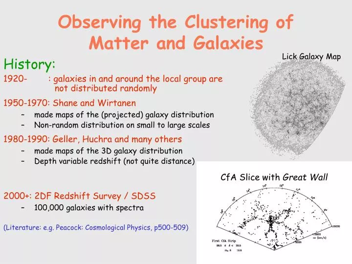
Lick Galaxy Map. CfA Slice with Great Wall. Observing the Clustering of Matter and Galaxies. History: 1920- : galaxies in and around the local group are not distributed randomly 1950-1970: Shane and Wirtanen made maps of the (projected) galaxy distribution

E N D
Lick Galaxy Map CfA Slice with Great Wall Observing the Clustering of Matter and Galaxies History: 1920- : galaxies in and around the local group are not distributed randomly 1950-1970: Shane and Wirtanen • made maps of the (projected) galaxy distribution • Non-random distribution on small to large scales 1980-1990: Geller, Huchra and many others • made maps of the 3D galaxy distribution • Depth variable redshift (not quite distance) 2000+: 2DF Redshift Survey / SDSS • 100,000 galaxies with spectra (Literature: e.g. Peacock: Cosmological Physics, p500-509) Vatican 2003 Lecture 20 HWR
Star-Forming Galaxies Red Galaxies State-of-the-Art Example: 2DFRS(from Peacock et al 2002) Vatican 2003 Lecture 20 HWR
Describing the Statistics of Clustering • There is no unique way to describe clustering! • Need to describe the degree of clustering not the particular configuration. • Isotropy: clustering = f(x,y,z) f(r) • Often-used measures are: • Angular or real-space correlation function • Genus curve • Smooth galaxies on different scales • Which fraction of the volume is filled by curves of a given over-/under-density • Counts-in cells • Main practical problems/issues: • Complicated search volumes • Finite number of tracers • Redshift space distortion Vatican 2003 Lecture 20 HWR
Correlation Functions • Excess probability of finding one galaxy (mass element) “near” another galaxy: - for a random (uniform) distribution: dP = n dV n: mean number density - a clustered distribution can be (incompletely) described by: dP(r) = n [1 + (r)] dV, where dP is the probability of finding a second object near an object at r = 0 (r): two-point (or, auto-) correlation function Note: (r) = < (x) (x+r) >, where (x) is the fractional over/under-density - to account for translation and rotation invariance (cosmological principle) often the Fourier transform is used P(k) | k|2 = (r) eikr d3r P(k): power spectrum - practical estimation: Vatican 2003 Lecture 20 HWR
If no redshifts (distances) are available, one can define the angular correlation function dP () = n (1 + w() ) d • Note: • understanding the sampling window function of a survey is crucial • usually one is measuring the correlation of tracers Vatican 2003 Lecture 20 HWR
Red galaxies Blue galaxies „Redshift“ Distance Angle on the sky The Clustering of Galaxies in the Present Day Universe (from the 2DFRS) • Redshift-space correlation Vatican 2003 Lecture 20 HWR
Axis ratio of the correlation in the space-velocity plane as a function of scale Infall Finger-of-God Finger-of-God and Inflow Signature • pairwise velocity dispersion from “finger-of-god”: 400km/s • Cosmic density estimate from inflow: b = W0.6/b = 0.43 0.07 Vatican 2003 Lecture 20 HWR
From Peacock et al 2002 More luminous/massive galaxies are more strongly clustered Galaxy Clustering vs. Galaxy Properties • Galaxies with little star-formation (~ “early types”) are much more strongly clustered on small scales • A.k.a. morphology-density relation • Presumably:dense environments lead to rapid/early completion of the main star-formation Vatican 2003 Lecture 20 HWR
Baryon wiggles? Cosmological Parameters from the Clustering of (Nearby) Galaxies Galaxy correlation now reflects: • initial fluctuations • growth rate (enter W and L) • transfer-function • Galaxy bias Comparison most straightforward in the linear regime >5-10 Mpc Vatican 2003 Lecture 20 HWR
Mass/Galaxy Clustering at high Redshift • Can one observe the growth of mass fluctuation and galaxy clustering directly? • Put a “point” between the CMB and the present epoch. • Two possible probes at z~3: • Galaxies (Ly-break galaxies) • The fluctuation inter-galactic medium (IGM): Ly-alpha forest • Galaxies:from Adelberger, Steidel and collaborators: • Ly-break galaxies at z~3 are nearly as clustered as L* galaxies now • (massive) galaxies were more biased tracers of the mass fluctuations than they are now. Vatican 2003 Lecture 20 HWR
The Ly-alpha Forest and Mass Fluctuations • What causes the fluctuation Ly-alpha absorption? • Collapsed objects (mini halos) • General density (+velocity) fluctuations Vatican 2003 Lecture 20 HWR
Simulating the Ly-alpha forest(Cen, Ostriker, Miralda 1994-; Croft, Katz, Weinberg, Hernquist 1996-) • Much of the Ly-alpha forest arises from modest density fluctuations and convergent velocity flows!! Vatican 2003 Lecture 20 HWR
From Croft et al 1998 Comparing Data and Simulations Vatican 2003 Lecture 20 HWR
The Correlation of IGM Absorptionat different redshifts • This probes the mass between galaxies • One can follow the evolution of structure with redshift Vatican 2003 Lecture 20 HWR
z=1100 z=0-3 Verde 2003 Combining the CMB with the low-z Universe • Until the last few years (BOOMERANG, MAXIMA, WMAP), the CMB fluctuations were measured on larger (co-moving) scales than the fluctuations measured in the low-z universe • Only joint extrapolation in redshift and scale possible! With new generation of z<5 LSS measurements and CMB experiments, a much more direct comparison is possible. Impressive confirmation of structure growth prediction!! Vatican 2003 Lecture 20 HWR
Joint Constraintsfrom large scale structure and the CMB • Note: • this is pre-WMAP, I.e. data from COBE + ground-based and baloon experiments! (from Peacock et al 2003) • h H0=100 Vatican 2003 Lecture 20 HWR
Theory Big Bang Inflation FRW/cosmological parameters WM=0.27,L=0.7,H0=70 (Non-baryonic) dark matter dominates (small) initial fluctuations Growth of density fluctuations Linear Observations Expansion,CMB,BBN Space is flat, CMB is uniform, fluctuations are scale free SN Ia, Galaxy Clustering, CMB Dynamics,lensing,BBN,CMB CMB CMB vs large-scale structure IGM fluctuations Galaxy large scale struture Let’s Recapitulate Vatican 2003 Lecture 20 HWR
Theory Non-linear growth of densities N-body,Press-Schechter (dark matter) halo profiles Hierarchical build-up of Structures Successive conversion of gas into stars Cooling, Feed-back Enrichment Remaining hot gas in clusters and IGM Observations Abundance, stellar mass and clustering of galaxies dynamics, lensing Observed merging, fewer massive galaxies at high-z(?) Recapitulation II Vatican 2003 Lecture 20 HWR
Observations Global star-formation history and QSO evolution(z>6 to now) Galaxy luminosity function and colors (as function of z) Morphologies, Bulge/Disk, etc f(z) vs. mass vs. environment Typical Sizes Global Scaling Relations Fundamental plane, Tully-Fisher MBH – s relation Theory Hierarchical merging and gas supply Gas cooling, feed-back, cold gas supply Gas Disks Merging Spheroids Hierarchical picture Hierarchical picture Angular momentum (but is it lost?) Constant star fraction; similar ang.mom. Good thing to work on… Galaxy Properties Recapitulation Vatican 2003 Lecture 20 HWR