Download
1 / 21
210 likes | 294 Views
A Hidden Markov Model for Progressive Multiple Alignment. Ari L ö ytynoja and Michel C. Milinkovitch Appeared in BioInformatics, Vol 19, no.12 , 2003 Presented by Sowmya Venkateswaran April 20,2006. Outline. Motivations Drawbacks of existing methods System and Methods Substitution Model

E N D
A Hidden Markov Model for Progressive Multiple Alignment Ari Löytynoja and Michel C. Milinkovitch Appeared in BioInformatics, Vol 19, no.12 , 2003 Presented by Sowmya Venkateswaran April 20,2006
Outline • Motivations • Drawbacks of existing methods • System and Methods • Substitution Model • Hidden Markov Model • Pairwise Alignment using Viterbi Algorithm • Posterior Probability • Multiple Alignment • Results • Discussion
Motivation • Progressive alignment techniques are used for Multiple Sequence Alignment • Used to deduce the phylogeny. • Identify protein families. • Probabilistic methods can be used to estimate the reliability of global/local alignments.
Drawbacks of existing Systems • Iterative application of global/local pairwise sequence alignment algorithms does not guarantee a globally optimum alignment. • A best scoring alignment may not correspond with true alignment. Hence reliability of a score/alignment needs to be inferred.
System and Methods • The idea is to provide a probabilistic framework for a guide tree and define a vector of probabilities at each character site. • Guide tree is constructed by using Neighbor Joining Clustering after producing a distance matrix. It can also be imported from CLUSTALW. • At each internal node, a probabilistic alignment is performed. Pointers from parent to child sites are stored and so also is a vector of probabilities of the different character states( ‘A/C/T/G/-’ for nucleotides or the 20 amino acids with a gap)
Substitution Model • Consider 2 sequences x1…nand y1…m, whose alignment we would like to find and their parent in the guide tree is z1…l. • Pa(xi) is the probability that site xi contains character a. Pa(xi) = 1, if a character a appears at terminal node, else it is 0. • At internal nodes, different characters have different probabilities summing to 1. • If the observed character is ambiguous, probability is shared among different characters.
Emission Probabilities Pxi,yj represents the probability that xi and yj are aligned. pxi,yj=pzk(xi,yj)=∑pzk=a(xi,yj) Pzk=a(xi,yj)=qa∑bsabpb(xi)∑bsabpb(yj) qa is the character background probability sab, probability of aligning characters a and b, is calculated with the Jukes Cantor Model sab=1/n + (n-1)/n * e –(n/n-1) v when a=b sab=1/n - 1/n * e –(n/n-1) v when a≠b n is the size of the alphabet , v is the NJ-estimated branch length
Probabilities • To find pxi,- , the probability that zk evolved to a character on one of the child sites and a gap on the other child is pzk=a(xi,-)=qa∑bsabpb(xi)sa- The same applies for pxi,-. sa- is computed just like sab. • Any other model can be used for calculation of sab, instead of the Jukes Cantor Model. Ex: PAM (20 X 20) substitution matrix can be modified to include gaps and transformed to a (21X21) matrix, and the substitution probabilities can be derived from that.
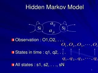
Hidden Markov Model X pxi,- ε δ 1-ε 1-2δ M pxi,yj 1-ε δ Y p-,yj ε
Hidden Markov Model • δ – probability of moving to an insert state (gap opening penalty) ; lower the value, higher the penalty. • ε – probability of staying at an insert state (gap extension penalty); again, lower the value, more the extension penalty. • pxi,yj ,pxi,- , p-,yj –emission frequencies for match, insert X and insert Y states. • For testing purposes, δ and ε were estimated from pairwise alignments of terminal sequences such that δ=1/2(lm+1) and ε=1-1/(lg+1); lm and lg are the mean lengths of match and gap segments.
Pairwise Alignment • In this probabilistic model, the best alignment between 2 sequences corresponds to the Viterbi path through the HMM. • Since there are 3 states in the model, and each state needs 2-D space, we have 3 2-D tables : vM for match states, vX and vY for the gap states. • A move within M, X or Y tables produces an additional match or extends an existing gap. A move between M table and either X or Y table closes or opens a gap.
Viterbi Recursion Initialization: v(0,0) = 1, v(i,-1) = v(-1,j)=0 Recursion: vM(i,j) = pxi,yj max { (1-2δ) vM(i-1,j-1), (1-ε) vX(i-1,j-1), (1-ε) vY(i-1,j-1) } vX(i,j) = pxi,- max { δvM(i-1,j), εvX(i-1,j) } vY(i,j) = p-,yj max { δvM(i,j-1), εvY(i,j-1) } Termination: vE=max(vM(n,m),vX(n,m),vY(n,m))
Viterbi traceback • At each cell, the relative probabilities of entering the different cells are stored. Ex: pM-M= (1-2δ) vM(i-1,j-1)/N(i,j) where N(i,j) is the normalizing constant, given by N(i,j)=(1-2δ) vM(i-1,j-1)+(1-ε)*[vX(i-1,j-1)+ vY(i-1,j-1)] The above equation is calculated for each of the 3 tables • Trace back algorithm used to find the best path; a match step will create pointers from the parent site to the child sites, and a gap step will create pointer to one and a gap for the 2nd child site.
Posterior Probabilities-Forward algorithm Forward algorithm-sum of probabilities of all paths entering a given cell from the start position. Initialization: f(0,0)=1;f(i,-1)=f(-1,j)=0; Recursion: i=0,…,n j=0,…,m, except (0,0) fM(i,j) = pxi,yj [ (1-2δ) fM(i-1,j-1) + (1-ε) ( fX(i-1,j-1)+ fY(i-1,j-1))] fX(i,j) = pxi,- [ δ fM(i-1,j) + ε fX(i-1,j)] fY(i,j) = p-,yj [ δ fM(i,j-1) + ε fY(i,j-1)] Termination: fE=fM(n,m)+fX(n,m)+fY(n,m)
Backward algorithm Sum of probabilities of all possible alignments between subsequences xi…n and yj…m. Initialization: b(n,m)=1; b(i,m+1) = f(n+1,j) = 0; Recursion: i=n,…,1 j=m,…,1, except (n,m) bM(i,j) = (1-2δ) px(i+1),y(j+1) bM(i+1,j+1) + δ [ px(i+1),- bX(i+1,j) + p-,y(j+1) bY(i,j+1)] bX(i,j) = (1-ε) px(i+1),y(j+1) bM(i+1,j+1) + ε px(i+1),- bX(i+1,j) bY(i,j) = (1-ε) px(i+1),y(j+1) bM(i+1,j+1) + ε p-,y(j+1) bX(i+1,j)
Reliability Check • Assumption: Posterior probability of the sites on the alignment path is a valid estimator of the local reliability of the alignment since it gives the proportion of total probability corresponding to all alignments passing through the cell (i,j). • Posterior probability for a match is given by: P(xi◊yj|x,y) = fM(i,j) bM(i,j) / fE where fM and bM are the total probabilities of all possible alignments between subsequences x1…i and y1…j and xi…n and yj…m respectively Similar probabilities are calculated for Insert X and Insert Y states too.
Multiple alignment • Each parent node site has a vector of probabilities corresponding to each possible character state (including the gap). For a match, pa(zk)=pzk=a(xi,yj)/∑bpzk=b(xi,yj) • Pairwise alignment builds the tree progressively, from the terminal nodes towards an arbitrary root. • Once root node is defined, trace-back is done to find multiple alignment of the nodes below since each node stores pointers to the matching child sites. • If a gap occurs in one of the internal nodes, a gap character state is introduced in all of the sequences of that sub-tree, and recursive call will not proceed further in that branch.
Testing • Algorithms tested on (i) simulated nucleotide sequences 50 random data sets generated using the program Rose. A root random sequence (length 500) was evolved on a random tree to yield sequences of “low” (no. of substitutions per site 0.5) and “high” (1.0) divergences. Also, the insertion/deletion length distribution was set to ‘short’ or ‘long’. (ii) Amino acid data sets from Ref1 of the BAliBASE database. Ref1 contains alignments of less than 6 equi-distant sequences, i.e., the percent-identity between 2 sequences is within a specified range with no large insertion or deletion. Datasets were divided into 3 groups based on lengths, and further into 3 based on similarities.
Performance and Future Work • ProAlign performs better than ClustalW for the nucleotide sequences, but not for amino acid sequences with sequence identity less than 25%. • Possible reasons may be that the model does not take into account, the protein secondary structure. So, the HMM can be extended to modeling protein secondary structure too. • Minimum posterior probability correlates well with correctness ; can be used to detect/remove unreliably aligned regions