Download
1 / 32
340 likes | 444 Views
3D Sensing and Mapping. B659: Principles of Intelligent Robot Motion Spring 2013 Kris Hauser. Agenda. A high-level overview of visual sensors and perception algorithms Core concepts Camera / p rojective geometry Point clouds Occupancy grids Iterative closest points algorithm.

E N D
3D Sensing and Mapping B659: Principles of Intelligent Robot Motion Spring 2013 Kris Hauser
Agenda • A high-level overview of visual sensors and perception algorithms • Core concepts • Camera / projective geometry • Point clouds • Occupancy grids • Iterative closest points algorithm
Proprioceptive: sense one’s own body • Motor encoders (absolute or relative) • Contact switches (joint limits) • Inertial: sense accelerations of a link • Accelerometers • Gyroscopes • Inertial Measurement Units (IMUs) • Visual: sense 3D scene with reflected light • RGB: cameras (monocular, stereo) • Depth: lasers, radar, time-of-flight, stereo+projection • Infrared, etc • Tactile: sense forces • Contact switches • Force sensors • Pressure sensors • Other • Motor current feedback: sense effort • GPS • Sonar
Sensing vs Perception • Sensing: acquisition of signals from hardware • Perception: processing of “raw” signals into “meaningful” representations • Example: • Reading pixels from a camera is sensing. • Declaring “it’s a rounded shape with skin color”, “it’s a face”, or “it’s a smiling face” are different levels of perception. • Especially at lower levels of perception like signal processing, the line is blurry, and the often the processed results can be essentially considered “sensed”. Digits
3D Perception Topics • Sensors: visible-light cameras, depth sensors, laser sensors • (Some) perception tasks: • Stereo reconstruction • Object recognition • 3D mapping • Object pose recognition • Key issues: • How to represent and optimize camera transforms? • How to fit models in the presence of noise? • How to represent large 3D models?
Visual Sensors • Visible-light cameras: cheap, low power, high resolution, high frame rates • Data: 2D field of RGB pixels • Stereo cameras • Depth field sensors • Two major types: infrared pattern projection (Kinect, ASUS, PrimeSense) and time-of-flight • Data: 2D field of depth values (SwissRanger) • Sweeping laser sensors • Data: 1D field of depth values • Hokuyo, SICK, Velodyne • Can be mounted on a tilt/spin mount to get 3D field of view Bumblebee stereo camera ASUS Xtion depth sensor Hokuyo laser sensor
Sensors vary in strengths / weaknesses • Velodyne (DARPA grand challenge) • 1.3 million readings/s • $75k price tag
Image formation • Light bounces off an object, passes through a lens and lands on a CCD pixel on the image plane • Depth of focus • Illumination and aperture • Color: accomplished through useof filters, e.g. Bayer filter • Each channel’s in-between pixels are interpolated
Idealized projective geometry • Let: • Zim: distance from image plane to focal point along the depth axis • (X,Y,Z): point in 3D space relative to focal point, Z > 0 • Then, image space point is: • Xc= Zim X / Z • Yc = Zim Y / Z …Which get scaled and offset to getpixel coordinates x Image plane (X,Z) (Xc,Zim) Focal point z
Issues with real sensors • Motion blur • Distortion caused by lenses • Non-square pixels • Exposure • Noise • Film grain • Salt-and-pepper noise • Shot noise Motion blur Distortion Exposure
Calibration • Determine camera’s intrinsic parameters • Focal length • Field of view • Pixel dimensions • Radial distortion • That determine the mapping from image pixels to an idealized pinhole camera • Rectification
Stereo vision processing • Dense reconstruction • Given two rectified images, find binocular disparity at each pixel • Take a small image patch around each pixel in the left image, search for the best horizontal shifted copy in the right image • What size patch? What search size? What matching criterion? • Works best for highly textured scenes
Point Clouds • Unordered list of 3D points P={p1,…,pn} • Each point optionally annotated by: • Color (RGB) • Sensor reading ID# (why?) • Estimated surface normal (nx,ny,nz) • No information about objects, occlusions, topology • Point Cloud Library (PCL) • http://pointclouds.org
3D Mapping • Each frame of a depth sensor gives a narrow snapshot of the world geometry from a given position • 3D mapping is the process of stitching multiple views into a global model
Three scenarios: • Consider two raw point clouds P1 and P2 from cameras with transformations T1 and T2. • Goal: build point cloud P in frame T1 (assume identity) • Case 1: relative transformations known • Simple union P= P1 (T2-1 P2) • Case 2: small transformation • Pose registration problem • Vast majority of points correspond between scenes • Case 3: large transformation • Significant fraction of points do not correspond, lighting differences, more occlusions • Pose registration must be more robust to outliers
Case 2: Small transformations • Visual odometry: estimate relative motion of subsequent frames using optical flow • Define feature points in P1 (e.g., corner detector) • Estimate a transformation of an image patch around feature that best matches P2 (defines optical flow field) • Transformation: translation, rotation, scale • Fit T2to match these feature transforms
Case 3: Large transformations • Iterative closest point algorithm • Input: initial guess for T2 • Repeat until convergence: • Find nearest neighbor pairings between P1 and T2P2 • Select those pairs that fall below some distance threshold (outlier rejection) • Assign an error metric and optimize T2 to minimize this metric
Case 3: Large transformations • Iterative closest point algorithm • Input: initial guess for T2 • Repeat until convergence: • Find nearest neighbor pairings between P1 and T2P2 • Select those pairs that fail to satisfy some distance criteria (outlier rejection) • Assign an error metric and optimize T2 to minimize this metric What metric? What criteria? How to minimize?
What metrics for matching? • Position • Surface normal • Color • Nearest neighbor methods • Fast data structures, e.g. K-D trees • For large scans usually want a constant sized subsample • Projection-based methods • Render scene from perspective of T1to determine a match • Very fast (used in Kinect Fusion algorithm) • Only uses position information
What criteria for outlier rejection? • Distance too large (e.g., top X%) • Inconsistencies with neighboring pairs • On boundary of scan
How to optimize? • Want to find rotation R, translation t of T2 to minimize some error function • Sum of squared point-to-point differences • Closed-form solution (SVD) • Very fast per step • Sum of squared point-to-plane differences • Must use numerical methods • Deal with rotation variable • Tends to lead ICP to converge with fewer iterations
Other applications of ICP • Fitting 3D triangulated models to point clouds for object recognition / pose estimation
Stitching multiple scans • In its most basic form, multi-view 3D mapping is simply a repetition of the two-camera case • But two major issues: • Drift and “closing the loop” • Point clouds become massive after many scans This time
Point cloud growth problem • With N points, at F frames/sec, and T seconds of run time, NFT points are gathered • Kinect: N=307200, F=30, T=60 => 552,960,000 points • With RGB in 4 bytes, XYZ in 12 bytes => 8 GB / min • Solutions: • Forget earlier scans (short term memory) • Build persistent, “collapsed” representation of environment geometry • Polygon meshes • Occupancy grids • Key issue: how to estimate with low # of points and update later?
Occupancy grids • Store a grid G with a fixed minimum resolution • Mark which cells (voxels) are occupied by a point • Representation sizeis independent of T • Two options for updating on a new scan • Compute ICP to align current scan to prior scan, then add points to G • Modify ICP to work directly with the representation G
Probabilistic Occupancy Grids with Ray Casting • Scans are noisy, so simply adding points is likely to overestimate occupied cells • Ray casting approaches: • Each cell has a probability of being free/occupied/unseen • Each scan defines a line segment that passes through free space and ends in an occupied cell (or near one) • Walk along the segment, increasing P(free(c)) of each encountered cell c, and finally increase P(occupied(c)) for the terminal cell c
Probabilistic Occupancy Grids with Ray Casting • Scans are noisy, so simply adding points is likely to overestimate occupied cells • Ray casting approaches: • Each cell has a probability of being free/occupied/unseen • Each scan defines a line segment that passes through free space and ends in an occupied cell (or near one) • Walk along the segment, increasing P(free(c)) of each encountered cell c, and finally increase P(occupied(c)) for the terminal cell c
Compact geometry representations within a cell • On-line averaging • On-line least squares estimation of fitting plane
Handling large 3D grids • Problem: tabular 3D grid storage increases with O(N3) • 10243 is 1Gb • Solutions • Store hash table only of occupied cells • Octree data structure • OctoMap Library (http://octomap.sourceforge.net)
Dynamic Environments • Real environments have people, animals, objects that move around • Two options: • Map static parts by assuming dynamic objects will average out as noise over time (probabilistic occupancy grids) • Segment (and possibly model) dynamic objects
Related topics • Sensor fusion • Object segmentation and recognition • Simultaneous Localization and Mapping (SLAM) • Next-best-view planning
Next time • Kalman filtering • Welch and Bishop (2001) • Principles Ch. 8 • Zeeshan