Download
1 / 24
240 likes | 321 Views
Section 8.2 Basics of Hypothesis Testing. Objective For a population parameter ( p, µ, σ ) we wish to test whether a predicted value is close to the actual value (based on sample values). In statistics, a Hypothesis is a claim or statement about a property of a population.

E N D
Section 8.2Basics of Hypothesis Testing Objective For a population parameter (p, µ, σ) we wish to test whether a predicted value is close to the actual value (based on sample values).
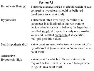
In statistics, a Hypothesis is a claim or statement about a property of a population. A Hypothesis Test is a standard procedure for testing a claim about a property of a population. Ch. 8 will cover hypothesis tests about a Proportion p Mean µ (σ known or σ unknown) Standard Deviation σ Definitions
Example 1 Claim: The XSORT method of gender selection increasesthe likelihood of birthing a girl. (i.e. increases the proportion of girls born) To test the claim, use a hypothesis test (about a proportion) on a sample of 14 couples: If 6 or 7 have girls, the method probably doesn’t increasethe probability of birthing a girl. If 13 or 14 couples have girls, this method probably does increase the probability of birthing a girl. This will be explained in Section 8.3
Rare Event Rule forInferential Statistics If, under a given assumption, the probability of a particular event is exceptionally small, we conclude the assumption is probably not correct. Example: Suppose we assume the probability of pigs flying is 10-10 If we find a farm with 100 flying pigs, we conclude our assumption probably wasn’t correct
Components of aHypothesis Test Null Hypothesis: H0 Alternative Hypothesis: H1
The null hypothesis(denoted H0) is a statement that the value of a population parameter (p, µ, σ) isequal tosome claimed value. We test the null hypothesis directly. It will either reject H0or fail to reject H0 (i.e. accept H0) Null Hypothesis: H0 ExampleH0: p = 0.6 H1: p < 0.6
Alternative Hypothesis: H1 The alternative hypothesis (denoted H1) is a statement that the parameter has a value that somehow differs from the null hypothesis. The difference will be one of <, >, ≠ (less than, greater than, doesn’t equal) ExampleH0: p = 0.6 H1: p < 0.6
Example 1 • Claim: The XSORT method of gender selection • increasesthe likelihood of birthing a girl. • Let p denote the proportion of girls born. • The claim is equivilent to “p>0.5” The null hypothesis must say “equal to”: H0: p = 0.5 The alternative hypothesis states the difference: H1: p > 0.5 Here, the original claim is the alternative hypothesis
Example 1 Continued Claim: The XSORT method of gender selection increasesthe likelihood of birthing a girl. If we reject the null hypothesis, then the original clam is accepted. Conclusion: The XSORT method increases the likelihood of having a baby girl. If we fail to reject the null hypothesis, then the original clam is rejected. Conclusion: The XSORT method does not increase the likelihood of having a baby girl. Note: We always test the null hypothesis
Example 2 • Claim: For couples using the XSORT method, the likelihood of having a girl is 50% • Again, let p denote the proportion of girls born. • The claim is equivalent to “p=0.5” The null hypothesis must say “equal to”: H0: p = 0.5 The alternative hypothesis states the difference: H1: p ≠ 0.5 Here, the original claim is the null hypothesis
Example 2 Continued Claim: For couples using the XSORT method, the likelihood of having a girl is 50% If we reject the null hypothesis, then the original clam is rejected. Conclusion: For couples using the XSORT method, the likelihood of having a girl is not 0.5 If we fail to reject the null hypothesis, then the original clam is accepted. Conclusion: For couples using the XSORT method, the likelihood of having a girl is indeed 0.5 Note: We always test the null hypothesis
Example 3 • Claim: For couples using the XSORT method, the likelihood of having a girl is at least 50% • Again, let p denote the proportion of girls born. • The claim is equivalent to “p ≥ 0.5” The null hypothesis must say “equal to”: H0: p = 0.5 The alternative hypothesis states the difference: H1: p < 0.5 Here, the original claim is the null hypothesis we can’t use ≥ or ≤ in the alternative hypothesis, so we test the negation
Example 3 Continued Claim: For couples using the XSORT method, the likelihood of having a girl is at least 50% If we reject the null hypothesis, then the original clam is rejected. Conclusion: For couples using the XSORT method, the likelihood of having a girl is less than 0.5 If we fail to reject the null hypothesis, then the original clam is accepted. Conclusion: For couples using the XSORT method, the likelihood of having a girl is at least 0.5 Note: We always test the null hypothesis
General rules • If the null hypothesis is rejected, the alternative hypothesis is accepted. H0 rejected → H1 accepted • If the null hypothesis is accepted, the alternative hypothesis is rejected. H0 accepted → H1rejected • Acceptance or rejection of the null hypothesis is called an initial conclusion. • The final conclusion is always expressed in terms of the original claim. Not in terms of the null hypothesis or alternative hypothesis.
A Type I erroris the mistake of rejecting the null hypothesis when it is actually true. Also called a “True Negative”True: means the actual hypothesis is trueNegative: means the test rejected the hypothesis The symbol (alpha) is used to represent the probability of a type I error. Type I Error
A Type II erroris the mistake of acceptingthe null hypothesis when it is actually false. Also called a “False Positive”False: means the actual hypothesis is falsePositive: means the test failed to reject the hypothesis The symbol (beta) is used to represent the probability of a type II error. Type II Error
Example 4 • Claim: A new medication has greater success rate (p) than that of the old (existing) machine (p0) • p: Proportion of success for the new medication • p0: Proportion of success for the old medication • The claim is equivalent to “p > p0” Null hypothesis: H0: p = p0 Alternative hypothesis:H1: p > p0 Here, the original claim is the null hypothesis
Example 4 Continued Claim: A new medication has greater success rate (p) than that of the old (existing) machine (p0) H0: p = p0 H1: p > p0 Type I error H0 is true, but we reject it → We accept the claim So we adopt the new (inefficient, potentially harmful) medicine. (This is called a critical error, must be avoided) Type II error H1 is true, but we reject it → We reject the claim So we decline the new medicine and continue with the old one. (no direct harm…)
Significance Level • The probability of a type I error (denoted ) is also called the significance level of the test. • Characterizes the chance the test will fail.(i.e. the chance of a type I error) • Used to set the “significance” of a hypothesis test.(i.e. how reliable the test is in avoiding type I errors) • Lower significance → Lower chance of type I error • Values used most: = 0.1, 0.05, 0.01 (i.e. 10%, 5%, 1%, just like with CIs)
Critical Region Consider a parameter (p, µ, σ, etc.) The “guess” for the parameter will have a probability that follows a certain distribution (z, t, χ2,etc.) Note: This is just like what we used to calculate CIs. Using the significance levelα, we determine the region where the guessed value becomes unusual. This is known as the critical region. The region is described using critical value(s).(Like those used for finding confidence intervals)
Example p follows a z-distribution If we guess p > p0 the critical region is defined by the right tail whose area is α If we guess p < p0 the critical region is defined by the left tail whose area is α If we guess p ≠ p0 the critical region is defined by the two tails whose areas areα/2 tα -tα -tα/2 tα/2
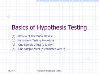
Testing a Claim Using a Hypothesis Test • 1. State the H0 and H1 • 2. Compute the test statistic • Depends on the value being tested • 3. Compute the critical region for the test statistic • Depends on the distribution of the test statistic (z, t, χ2) • Depends on the significance level α • Found using the critical values • 4. Make an initial conclusion from the test • RejectH0 (accept H1) if the test statistic is within the critical region • AcceptH0 if test statistic is not within the critical region • 5. Make a final conclusion about the claim • State it in terms of the original claim
Example 5 Claim: The XSORT method of gender selection increasesthe likelihood of birthing a girl. Suppose 14 couples using XSORT had 13 girls and 1 boy. Test the claim at a 5% significance level H0: p = 0.5 H1: p > 0.5 1. State H0 and H1 2.Find the test statistic 3.Find the critical region 4. Initial conclusion 5. Final conclusion We accept the claim