Download
1 / 33
330 likes | 477 Views
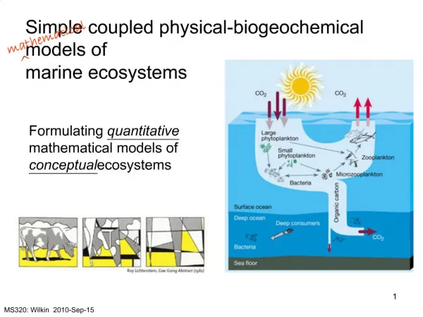
Physical and Biogeochemical Coupled Modelling. Presented by Christel PINAZO Mediterranean University Oceanographic Center of Marseille Physical & Biogeochemical Oceanographic Laboratory.

E N D
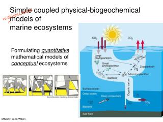
Physical and Biogeochemical Coupled Modelling Presented by Christel PINAZO Mediterranean University Oceanographic Center of Marseille Physical & Biogeochemical Oceanographic Laboratory Regional Advanced School on Physical and Mathematical Tools for the study of Marine Processes of Coastal Areas
LECTURE SCHEDULE • Introduction • Why use Coupled Models ? • Historical considerations • Different types of Coupled Models • Box models • Fine grid Models (1D, 2D and 3D) • Different ways of Coupling Models • « Off-line » Coupling • « On-line » Coupling • Examples
COUPLING TYPES THE STUDY SITE COULD BE SPATIALLY DESCRIBED BY FINE MESH GRID IN 1D, 2D OR 3D INTRODUCTION COUPLING TYPES>FINE COUPLING WAYS EXAMPLES Regional Advanced School on Physical and Mathematical Tools for the study of Marine Processes of Coastal Areas
COUPLING TYPES TO CALCULATE THE VARIATION OF BIOGEOCHEMICAL CONCENTRATIONS : - EQUATION OF TEMPERATURE VARIATION OF THE HYDRODYNAMIC MODEL INTRODUCTION COUPLING TYPES>FINE COUPLING WAYS EXAMPLES Regional Advanced School on Physical and Mathematical Tools for the study of Marine Processes of Coastal Areas
COUPLING TYPES z 1D FINE GRID MODEL (VERTICAL) z=0 h Time evolution Vertical advection Settling Velocity Vertical eddy diffusivity Concentration Trend term= Sources – Sinks z=-h SEDIMENT INTRODUCTION COUPLING TYPES>FINE COUPLING WAYS EXAMPLES Regional Advanced School on Physical and Mathematical Tools for the study of Marine Processes of Coastal Areas
COUPLING TYPES 1D FINE GRID MODEL (VERTICAL) ADVANTAGES: • FINE DISCRETISATION ONLY ALONG VERTICAL AXIS • SIMULATION OF VERTICAL EDDY DIFFUSIVITY (MIXED LAYER) AND UP OR DOWNWELLING PHENOMENA • RELATIVE SHORT COMPUTATIONAL TIME • LONG SIMULATION OF SEASONS OR YEARS DISADVANTAGES: • NOT SIMULATE HORIZONTAL ADVECTION • NOT SIMULATE CORIOLIS EFFECT INTRODUCTION COUPLING TYPES>FINE COUPLING WAYS EXAMPLES Regional Advanced School on Physical and Mathematical Tools for the study of Marine Processes of Coastal Areas
y O x COUPLING TYPES 2D FINE GRID MODEL (HORIZONTAL) depth-integrating Navier-Stokes equations Concentration Trend term= Sources – Sinks Time evolution Horizontal advection Horizontal eddy diffusivity INTRODUCTION COUPLING TYPES>FINE COUPLING WAYS EXAMPLES Regional Advanced School on Physical and Mathematical Tools for the study of Marine Processes of Coastal Areas
COUPLING TYPES 2D FINE GRID MODEL (HORIZONTAL) ADVANTAGES: • DISCRETISATION ONLY ALONG HORIZONTAL AXES • SIMULATION OF HORIZONTAL ADVECTION AND DIFFUSIVITY • SIMULATION OF CORIOLIS EFFECT • MEAN COMPUTATIONAL TIME • SIMULATION OF MONTHS OR SEASONS DISADVANTAGES: • NOT SIMULATE VERTICAL EDDY DIFFUSIVITY (MIXED LAYER) • NOT SIMULATE UP OR DOWNWELLING PHENOMENA • NOT SIMULATE SEVERAL-LAYERS INTRODUCTION COUPLING TYPES>FINE COUPLING WAYS EXAMPLES Regional Advanced School on Physical and Mathematical Tools for the study of Marine Processes of Coastal Areas
z y O x COUPLING TYPES 3D FINE GRID MODEL Navier-Stokes equations Concentration Trend term= Sources – Sinks Time evolution 3D advection 3D eddy diffusivity INTRODUCTION COUPLING TYPES>FINE COUPLING WAYS EXAMPLES Regional Advanced School on Physical and Mathematical Tools for the study of Marine Processes of Coastal Areas
COUPLING TYPES 3D FINE GRID MODEL ADVANTAGES: • FINE DISCRETISATION ALONG THE 3D AXES • SIMULATION OF ALL THE MAIN PHENOMENA DISADVANTAGES: • RELATIVE LONG COMPUTATIONAL TIME • SHORT SIMULATION OF FORTNIGTH TO MONTHS INTRODUCTION COUPLING TYPES>FINE COUPLING WAYS EXAMPLES Regional Advanced School on Physical and Mathematical Tools for the study of Marine Processes of Coastal Areas
LECTURE SCHEDULE • Introduction • Why use Coupled Models ? • Historical considerations • Different types of Coupled Models • Box models • Fine grid Models (1D, 2D and 3D) • Different ways of Coupling Models • « Off-line » Coupling • « On-line » Coupling • Examples
COUPLING WAYS • 2 • DIFFERENT COUPLING WAYS : • OFF-LINE : 2 SEPARATED RUNS WITH PHYSICAL FORCING CONDITIONS STORED IN FILES • ON-LINE : DIRECT AND DYNAMIC COUPLING IN 1 RUN INTRODUCTIONCOUPLING TYPES COUPLING WAYS EXAMPLES Regional Advanced School on Physical and Mathematical Tools for the study of Marine Processes of Coastal Areas
LECTURE SCHEDULE • Introduction • Why use Coupled Models ? • Historical considerations • Different types of Coupled Models • Box models • Fine grid Models (1D, 2D and 3D) • Different ways of Coupling Models • « Off-line » Coupling • « On-line » Coupling • Examples
Physical Forcing Variables : Currents Eddy diffusivity Surface elevation… dt = 50 s Physical Forcing Ecological trends Spatial and temporal evolution Of biogeochemical variables OFF-LINE COUPLING dt= 600 s Hydrodynamic Model MARS 3D Wind Tide Advection Diffusion Biogeochemical variables dt= 1200 s Ecological Model Eco3M dt= 1 hour Irradiance River inputs Wastewater inputs INTRODUCTIONCOUPLING TYPES COUPLING WAYS>OFF-LINE EXAMPLES Regional Advanced School on Physical and Mathematical Tools for the study of Marine Processes of Coastal Areas
DIRECT AND DYNAMIC COUPLING dt= 1 hour dt= 1200 s Ecological Model Irradiance River inputs Wastewater inputs Ecological trends dt= 50 s dt= 600 s Hydrodynamic Model Advection Diffusion variables bio Physical Variables : Currents Surface elevation… Wind Tide dt = 50 s Spatial and temporal evolution Of biogeochemical variables INTRODUCTIONCOUPLING TYPES COUPLING WAYS>ON-LINE EXAMPLES Regional Advanced School on Physical and Mathematical Tools for the study of Marine Processes of Coastal Areas
EXAMPLES 3D coupled physical and biogeochemical Modelling Study of ecosystem functioning Of the SW lagoon of New Caledonia INTRODUCTION COUPLING TYPES COUPLING WAYS EXAMPLES Regional Advanced School on Physical and Mathematical Tools for the study of Marine Processes of Coastal Areas
Nord Study site West wind Trade winds
Wind measurements (îlot Maître) Dumbéa river Inputs Direction, 360° Débit, m3 s-1 Vitesse, m s-1 Data from PhD thesis S. Jacquet (2005) Study site • High short-term variability of meteorological forcings • Low seasonal variability
Physical Modelling Mars3D ECO3M • horizontal mesh grid: 500m • Nb horizontal cells: 340*90 • 10 vertical sigma levels • Forcings : wind, tides Ecological Model: 170*90 Horizontal cells IFREMER-IRD (P. DOUILLET)
Physical Modelling NOUMÉA Surface currents: Trade winds 8 m s-1
Ecological Modelling • Current Model • C and N Cycles • 12 variables • Zooplankton • = « forcing function » • Eco3M tool
Ecological Modelling Faure et a (2006) Phytoplankton biomass measurements Phytoplankton biomass modelling ? Chl.a Carbon Nitrogen …. • Constant ratio Carbon : Chlorophyll a But: • Chl.a : diagnosticvariable calculated from other state variables • Chl.a : Dynamic state variable
Dynamic coupling between the 2 models dt= 1 hour dt= 1200 s Ecological Model Eco3M (LOB) Irradiance River inputs Wastewater inputs Ecological trends dt= 50 s dt= 600 s Hydrodynamic Model MARS 3D (IFREMER-IRD) Advection Diffusion variables bio Physical Variables : Currents Surface elevation… Wind Tide dt = 50 s Spatial and temporal evolution Of biogeochemical variables
Field measurements : HIVER 2003 Vent Irradiance Measured forcings Débit des rivières
Realistic Simulation : HIVER 2003, 2D Results Weak Trade winds Weak West wind Chla, µg l-1 19 June 3 July
Realistic Simulation : HIVER 2003, 2D Results West wind Trade Winds Chla, µg l-1 3 July 15 July
Realistic Simulation : HIVER 2003, 2D Results Trade Winds and rainfall Chla, µg l-1 15 July 26 July
Realistic Simulation : HIVER 2003, 2D Results West wind Trade winds Chla, µg l-1 26 July 7 August