Download
1 / 32
350 likes | 669 Views
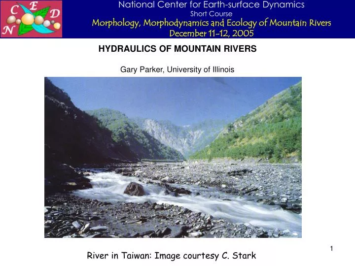
HYDRAULICS OF MOUNTAIN RIVERS Gary Parker, University of Illinois. River in Taiwan: Image courtesy C. Stark. TOPICS COVERED.

E N D
HYDRAULICS OF MOUNTAIN RIVERS Gary Parker, University of Illinois River in Taiwan: Image courtesy C. Stark
TOPICS COVERED • This lecture is not intended to provide a full treatment of open channel flow. Nearly all undergraduate texts in fluid mechanics for civil engineers have sections on open channel flow (e.g. Crowe et al., 2001). Three texts that specifically focus on open channel flow are those by Henderson (1966), Chaudhry (1993) and Jain (2000). • Topics treated here include: • Approximations for the channel • Shields number, Einstein number, generic bedload equation • Boundary resistance in mountain streams: Chezy and Manning-Strickler forms • Skin friction and form drag in mountain rivers • Backwater and the backwater length • Normal (steady, uniform) flow • Calculations of flow and sediment transport using the normal flow assumption
SIMPLIFICATION OF CHANNEL CROSS-SECTIONAL SHAPE River channel cross sections have complicated shapes. In a 1D analysis, it is appropriate to approximate the shape as a rectangle, so that B denotes channel width and H denotes channel depth (reflecting the cross-sectionally averaged depth of the actual cross-section). As was seen the lecture on hydraulic geometry, natural channels are generally wide in the sense that Hbf/Bbf << 1, where the subscript “bf” denotes “bankfull”. As a result the hydraulic radius Rh is usually approximated reasonably accurately by the average depth. In terms of a rectangular channel,
THE SHIELDS NUMBER: A KEY DIMENSIONLESS PARAMETER QUANTIFYING SEDIMENT MOBILITY b = boundary shear stress at the bed (= bed drag force acting on the flow per unit bed area) [M/L/T2] c = Coulomb coefficient of resistance of a granule on a granular bed [1] D = characteristic grain size (e.g. surface median size Ds50) Recalling that R = (s/) – 1, the Shields Number * is defined as It can be interpreted as scaling the ratio impelling force of flow drag acting on a bed particle to the Coulomb force resisting motion acting on the same particle, so that The characterization of bed mobility thus requires a quantification of boundary shear stress at the bed.
THRESHOLD OF MOTION IN MOUNTAIN STREAMS The threshold of motion is often expressed in terms of a Shields curve (Shields, 1936). Let denote the value of * at the threshold of motion, and Rep denote grain Reynolds number, defined in the lecture on hydraulic geometry as Based Neill’s (1968) work on coarse sedimentg, Parker et al. (2003) amended the Brownlie (1981) fit of the original Shields curve to the form The asymptotic value of for large Rep, i.e. coarse sediment, is 0.03. Consider the case of quartz (R = 1.65) in water at 20C ( = 1x10⁻⁶ m2/s). The smallest value of Ds50 for the data set introduced in the lecture on hydraulic geometry is 27 mm, in which case Rep = 17,850 and = 0.0289. So an approximate value of of 0.03 is appropriate for most coarse-bedded mountain streams. In point of fact, there is no sharply-defined threshold of motion. The value of 0.03 should be interpreted to be a value below which the bedload transport rate is morphodynamically insignificant, not precisely 0.
SHIELDS NUMBER AT BANKFULL FLOW IN MOUNTAIN STREAMS It will be shown in Slide 26 that for the case of mountain streams the Shields number at bankfull flow can be estimated as where all parameters were defined in the lecture on hydraulic geometry. A plot of versus is given to the right. The data are those from the lecture on hydraulic geometry. The average value of is 0.0486, i.e about 1.62 times the Shields number at the threshold of motion. Most alluvial gravel-bed streams move size Ds50 at bankfull flow.
THE EINSTEIN NUMBER: A DIMENSIONLESS QUANTIFICATION OF BEDLOAD TRANSPORT RATE qb = volume bedload transport rate per unit width [L2/T] D = characteristic grain size [L] R = (s/) – 1 1.65 for natural sediment [1] One standard approach to the quantification of bedload transport is the specification of the functional form An example appropriate for the bedload transport of gravel of uniform size is the modified form of the bedload transport equation of Meyer-Peter and Müller (1948) by Wong (2003): In field gravel-bed rivers, however, a) the gravel is rarely uniform and b) gravel is commonly transported at Shields numbers below 0.0495 (see previous slide).
BOUNDARY RESISTANCE IN MOUNTAIN STREAMS Let Q = flow discharge [L/T] B = water surface width [L] H = cross-sectionally averaged depth [L] U = Q/(BH) = cross-sectionally averaged flow velocity [L] u* = (b/)1/2 = shear velocity [L/T] Two dimensionless bed resistance coefficients are defined here: the Chezy resistance coefficient Cz given as and the standard bed resistance coefficient Cf (= f/8, where f denotes the D’arcy-Weisbach resistance coefficient); Note that as the bed shear stress increases, Cfincreases and Cz decreases.
RESISTANCE RELATIONS FOR HYDRAULICALLY ROUGH FLOW Mountain streams are almost invariably in the range of hydraulically rough flow, for which resistance becomes independent of kinematic viscosity . Keulegan (1938) offered the following relation for hydraulically rough flow. where ks = a roughness height characterizing the bumpiness of the bed [L]. A close approximation is offered by the Manning-Strickler formulation: Parker (1991) suggested a value of r of 8.1 for gravel-bed streams. The roughness height over a flat bed of coarse grains (no bedforms) is given as where Ds90 denotes the surface sediment size such that 90 percent of the surface material is finer, and nk is a dimensionless number between 1.5 and 3. For example, Kamphuis (1974) evaluated nk as equal to 2.
COMPARISION OF KEULEGAN AND MANNING-STRICKLER RELATIONS r = 8.1 Note that Cz does not vary strongly with depth. It is often approximated as a constant in broad-brush calculations.
TEST OF RESISTANCE RELATION AGAINST MOBILE-BED DATA WITHOUT BEDFORMS FROM LABORATORY FLUMES The data in question are from all the experiments without bedforms used by Meyer-Peter and Müller (1948) to develop their bedload relation. Here Rb denotes the bed component of hydraulic radius Rh rather than depth: the flumes were too narrow to allow the approximation Rh H.
FORM DRAG AND SKIN FRICTION The formulas of the previous slide hold only for flat, coarse granular beds. River beds are rarely flat. Lowland sand-bed streams typically contain dunes. Dunes are not common in mountain streams, but such bedforms as bars, pool-riffle sequences and step-pool sequences are common. All such features, as well as planform irregularity, contributed added resistance, so Cz is usually lower, and Cf is usually higher, than predicted by the equation of the previous slide. Step-pool pattern in the Hiyamizudani river, Japan. Cour. K. Hasegawa Bars in the Rhine River, Switzerland. Cour. M. Jaeggi
FORM DRAG AND SKIN FRICTION contd. The component of the resistance coefficient Cfs due to the flow acting on the grains themselves is known as skin friction, and the extra component Cff is denoted as form drag (due to bedforms), to that the total resistance coefficient Cf is given as Cfs can be computed from the relations of Slides 10 and 11. In bar-dominated mountain streams, form-drag is prominent at lower flows, but is muted at flood flows (see images to the right). In steeper streams with pool-riffle patterns, and in particular step-pool patterns, form drag is likely significant even at flood flows. Elbow River, Alberta, Canada at low flow and 100-year flood. Cour. Alberta Research Council
BACKWATER If (most) alluvial streams are disturbed at a point, the effect of that disturbance tends to propagate upstream. For example, the effect of a lake (slowing the flow down) or a waterfall (speeding the flow up) is felt upstream, as illustrated below. Backwater from a lake Backwater from a waterfall Backwater effects are mediated by a dimensionless number known as the Froude number Fr, where
BACKWATER contd. For most alluvial mountain streams, the Froude number at bankfull flow Frbf satisfies the condition As seen from the lecture on hydraulic geometry. For the case Fr < 1 backwater effects propagate upstream, so that the effect of a disturbance is felt upstream of it.
BACKWATER contd. Supercritical flow (Fr > 1) does occur in very steep mountain streams, and in particular streams with step-pool patterns and bedrock streams. In the case of a supercritical flow the effect of a disturbance propagates downstream rather than upstream. Stream in the interior of British Columbia, Canada. Cour. B. Eaton. Sustained supercritical flow over an alluvial or bedrock bed is unstable, and usually devolves into a series of steps punctuated by hydraulic jumps at formative flow. Dry Meadow Creek, Calif., USA. Cour. M. Neumann
THE BACKWATER LENGTH The characteristic distance Lb upstream (in the case of the more usual subcritical flow) or downstream (in the case of supercritical flow) to which the effect of a disturbance is felt is known as the backwater length. Let Hd = the flow depth at the disturbance [L] S = down-channel slope of the river [1]. The backwater length is then given as Taking Hb to scale with Hbf, some estimates of the backwater length are given below. Estimates of the backwater length obtained in this way average to 2.1 km, 1.1 km, 0.2 km, and 5.2 km for the data sets for Alberta, Britain, Idaho and Colorado introduced in the lecture on hydraulic geometry. That is, backwater lengths tend to be very short in mountain streams.
NORMAL FLOW Normal flow is an equilibrium state defined by a perfect balance between the downstream gravitational impelling force and resistive bed force, in the absence of any perturbation due to backwater. The resulting flow is constant in time and in the downstream, or x direction. The approximation of normal flow is often a very good one in mountain streams. • Parameters: • x = downstream coordinate [L] • H = flow depth [L] • U = flow velocity [L/T] • qw = water discharge per unit width [L2T-1] • B = width [L] • Qw = qwB = water discharge [L3/T] • g = acceleration of gravity [L/T2] • = bed angle [1] tb = bed boundary shear stress [M/L/T2] • S = tan = streamwise bed slope [1] • (cos 1; sin tan S) • = water density [M/L3] As can be seen from the lecture on hydraulic geometry, the bed slope S of most river, even most mountain rivers, is sufficiently small to allow the approximations
NORMAL FLOW contd. Conservation of water mass (= conservation of water volume as water can be treated as incompressible): Conservation of downstream momentum: Impelling force (downstream component of weight of water) = resistive force Reduce to obtain depth-slope product rule for normal flow:
CHEZY RESISTANCE COEFFICIENT AT BANKFULL FLOW Using the normal flow approximation, it is found between the relations that Cz can be estimated as Regression of all four data sets: This is how Czbf was estimated in the lecture on hydraulic geometry, as shown to the right. If Cz can be estimaged, the flow velocity U is then given as This relation is known as Chezy’s law.
MANNING-STRICKLER RESISTANCE RELATION FOR PLANE BED Using the normal flow approximation and the form for Cz for a plane bed in the absence of bedforms given in Slide 11, it is found that or solving for U, This is known as a Manning-Strickler resistance relation, where Manning’s “n” (a parameter that should be relegated to the dustbin due to its perverse dimensions) is given as (But you must remember to use MKS units for n, whereas the equation for U works for any consistent set of units).
MANNING-STRICKLER RESISTANCE RELATION FOR MOUNTAIN RIVERS AT BANKFULL FLOW The regression of the data of Slide 21 for mountain rivers at bankfull flow yields the relation where Ubf = Qbf/(HbfBbf), or thus This represents a generalized Manning-Strickler relation for mountain streams.
FORM DRAG VERSUS SKIN FRICTION AT BANKFULL FLOW In order to compare form drag versus skin friction at bankfull flow, it is necessary to estimate the roughness height ks. Here the Kamphuis (1974) relation Is used in conjunction with the reasonable estimate Then defining Cf,bf, Cfs,bf and Cff,bf as the values of the total resistance coefficient, the resistance coefficient due to skin friction and the resistance coefficient due to form drag, respectively at bankfull flow, it is found that The fraction of resistance that is form drag Fform is thus given as
FORM DRAG VERSUS SKIN FRICTION AT BANKFULL FLOW contd. The fraction of resistance that is form drag at bankfull flow in mountain streams is less than 0.5. The fraction is 0.2 ~ 0.3 in relatively deep mountain streams (Hbf/Ds50) > 20, but can be above 0.3 in relatively shallow mountain streams. Deeper streams tend to have lower slopes, and shallower streams tend to have higher slopes, as shown in the next slide.
SHIELDS NUMBER AT BANKFULL FLOW USING THE NORMAL FLOW ASSUMPTION Using the definition of the Shields number * and the estimate for bed shear stress b from the normal flow approximation, the following estimate is obtained for the Shields number at bankfull flow: This is the origin of the estimate of Shields number used in the chapter on hydraulic geometry and in Slide 7 of this lecture. A crude approximation of the plot to the right yields so that S decreases as Hbf/Ds50 increases.
CALCULATING THE FLOW AT NORMAL EQUILIBRIUM: CHEZY FORMULATION Between the relations it can be shown that Thus if the water discharge per unit width qw, down-channel bed slope S, characteristic bed grain size D and submerged specific gravity R are known, and if the Chezy resistance coefficient Cz can be estimated, the flow depth H, flow velocity U, bed shear stress b and Shields number * can be computed as indicated above.
CHEZY MANNING-STRICKLER For the case of plane-bed rough flow, the following formulation for resistance was given in Slide 10: The corresponding relation based on data for mountain rivers at bankfull flow is (Slide 20) Assuming that ks = 2 Ds90 and Ds90 = 3 Ds50, the above relation can be cast into the form Both relations can be cast in terms of a generalized Manning-Strickler formulation, such that
CALCULATING THE FLOW AT NORMAL EQUILIBRIUM: MANNING-STRICKLER FORMULATION Consider a generalized Manning-Strickler resistance relation of the form where for example g can be estimated as 5.92, ng can be estimated as 0.210 and ks can be estimated as 2Ds90 for mountain gravel-bed streams at flood flows (Slide 27). The relations for H, U, b and * now become where
CALCULATING BEDLOAD TRANSPORT AT NORMAL EQUILIBRIUM: For no particularly good reason, most formulations of bedload transport in gravel-bed streams have ignored form drag. For the sake of illustration, we do so here. Consider a “flume-like” river with no form drag and containing “uniform” gravel of size D, roughness height ks (~ 2D) and submerged specific gravity R. The reach has bed slope S, and is conveying water discharge per unit width qw. For this case it is reasonable to assume ng = 1/6 and g = 8.1, i.e. the relation of Slide 10. The Shields number can be computed from the previous slide as and the volume bedload transport rate per unit width q can be estimated from Slide 7 as
MANNING-STRICKLER: STANDARD CASE OF ng = 1/6: In the case of an exponent ng of 1/6 (the standard Manning-Strickler exponent of Slide 10), the relevant relations reduce to:
REFERENCES Brownlie, W. R., 1981, Prediction of flow depth and sediment discharge in open channels, Report No. KH-R-43A, W. M. Keck Laboratory of Hydraulics and Water Resources, California Institute of Technology, Pasadena, California, USA, 232 p. Chaudhry, M. H., 1993, Open-Channel Flow, Prentice-Hall, Englewood Cliffs, 483 p. Crowe, C. T., Elger, D. F. and Robertson, J. A., 2001, Engineering Fluid Mechanics, John Wiley and sons, New York, 7th Edition, 714 p. Gilbert, G.K., 1914, Transportation of Debris by Running Water, Professional Paper 86, U.S. Geological Survey. Jain, S. C., 2000, Open-Channel Flow, John Wiley and Sons, New York, 344 p. Kamphuis, J. W., 1974, Determination of sand roughness for fixed beds, Journal of Hydraulic Research, 12(2): 193-202. Keulegan, G. H., 1938, Laws of turbulent flow in open channels, National Bureau of Standards Research Paper RP 1151, USA. Henderson, F. M., 1966, Open Channel Flow, Macmillan, New York, 522 p. Meyer-Peter, E., Favre, H. and Einstein, H.A., 1934, Neuere Versuchsresultate über den Geschiebetrieb, Schweizerische Bauzeitung, E.T.H., 103(13), Zurich, Switzerland. Meyer-Peter, E. and Müller, R., 1948, Formulas for Bed-Load Transport, Proceedings, 2nd Congress, International Association of Hydraulic Research, Stockholm: 39-64. Neill, C. R., 1968, A reexamination of the beginning of movement for coarse granular bed materials, Report INT 68, Hydraulics Research Station, Wallingford, England. Parker, G., 1991, Selective sorting and abrasion of river gravel. II: Applications, Journal of Hydraulic Engineering, 117(2): 150-171.
REFERENCES Parker, G., Toro-Escobar, C. M., Ramey, M. and S. Beck, 2003, The effect of floodwater extraction on the morphology of mountain streams, Journal of Hydraulic Engineering, 129(11), 885-895. Shields, I. A., 1936, Anwendung der ahnlichkeitmechanik und der turbulenzforschung auf die gescheibebewegung, Mitt. Preuss Ver.-Anst., 26, Berlin, Germany. Vanoni, V.A., 1975, Sedimentation Engineering, ASCE Manuals and Reports on Engineering Practice No. 54, American Society of Civil Engineers (ASCE), New York. Wong, M., 2003, Does the bedload equation of Meyer-Peter and Müller fit its own data?, Proceedings, 30th Congress, International Association of Hydraulic Research, Thessaloniki, J.F.K. Competition Volume: 73-80. For more information see Gary Parker’s e-book: 1D Morphodynamics of Rivers and Turbidity Currents http://cee.uiuc.edu/people/parkerg/morphodynamics_e-book.htm