Download
1 / 40
400 likes | 533 Views
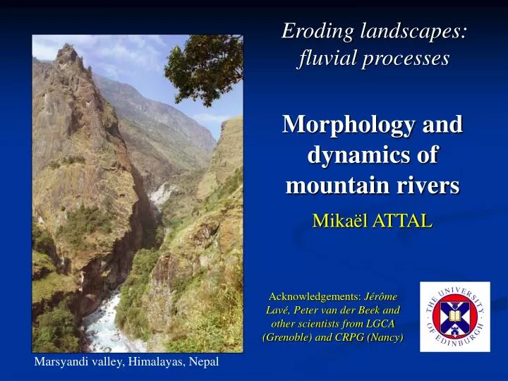
Eroding landscapes: fluvial processes. Morphology and dynamics of mountain rivers. Mikaël ATTAL. Acknowledgements: Jérôme Lavé, Peter van der Bee k and other scientists from LGCA (Grenoble) and CRPG (Nancy). Marsyandi valley, Himalayas, Nepal. Lecture overview.

E N D
Eroding landscapes: fluvial processes Morphology and dynamics of mountain rivers Mikaël ATTAL Acknowledgements: Jérôme Lavé, Peter van der Beek and other scientists from LGCA (Grenoble) and CRPG (Nancy) Marsyandi valley, Himalayas, Nepal
Lecture overview I. Morphology and geometry of mountain « bedrock » rivers II. Fluvial erosion laws: models and attempts of calibration
Erosion in mountains Glaciers and hillslope processes
Borrego badlands, California (www.parkerlab.bio.eci.edu) Southern Apennines, Italy Salerno Bryce Canyon, Utah (www.smugmug.com) 10 km Canyonlands National Park, Utah (Stu Gilfillan) RIVERS Cascade Mountains, California
In response to tectonic uplift, rivers incise into bedrock... http://projects.crustal.ucsb.edu/nepal/ Uplift Fluvial incision
… and insure the progressive lowering of the base level for hillslope processes http://projects.crustal.ucsb.edu/nepal/ Uplift Hillslope erosion
Rivers insure the transport of the erosion products to the sedimentary basin http://projects.crustal.ucsb.edu/nepal/ Dissolved load + suspended load + bed load
W S = 0.46W S Hierarchical organization of fluvial network Hovius, 1996, 2000
Hierarchical organization of fluvial network Hack’s law (1957) L = aAh L = length of stream a = constant h = constant in the range 0.5-0.6 in natural rivers Rigon et al., 1996
Hierarchical organization of fluvial network Response to active tectonics Galy, 1999
Hierarchical organization of fluvial network Response to active tectonics A: relay zone, large catchment, low subsidence rate B: fault “wall”, small catchments, large subsidence rate B A Tectonic control on drainage development (Eliet & Gawthorpe, 1995) B A
JGR, 2002 Hierarchical organization of fluvial network Response to active tectonics
Hierarchical organization of fluvial network Response to active tectonics Humphrey and Konrad, 2000
Development and evolution of river profiles Hovius, 2000
Development and evolution of river profiles Rivers adjust their SLOPES to increase or reduce erosion rates Uplift > Erosion Slope increases erosion increases until U = E (Steady-State). Steady-State means: rate of rock uplift relative to some datum, such as mean sea level, equals the erosion rate at every point in the landscape, so that topography does not change.
Development and evolution of river profiles Rivers adjust their SLOPES to increase or reduce erosion rates Uplift < Erosion Slope decreases erosion decreases until U = E (Steady-State). Steady-State means: rate of rock uplift relative to some datum, such as mean sea level, equals the erosion rate at every point in the landscape, so that topography does not change.
Mountain “bedrock” rivers EROSION DEPOSITION Sklar and Dietrich, 1998
Stream Power Law (SPL) Typical steady-state “concave-up” river profile: power law between slope and drainage area “Fluvial” bedrock channel θ “Debris-flow- dominated” bedrock channel S = KSA-θwhere KS = steepness index and θ = concavity index (0.5 ± 0.15) Debris-flow-dominated reaches: S independent of A, S controlled mostly by rock mass strength (angle of repose) Noyo River, California (Sklar and Dietrich, 1998)
S = KSA-θ KS is a function of uplift rate: high uplift high erosion rates needed to reach steady-state steep slopes needed. For a given A, the slope of a channel experiencing a high uplift rate (black) is higher than the slope of a channel experiencing low uplift rate (grey). log S log A San Gabriel Mts, California (Wobus et al., 2006)
NOTE: this applies to STEADY-STATE bedrock channels experiencing uniform uplift !!! Humphrey and Konrad, 2000 log S If uplift is not uniform or landscape is responding to a disturbance slopes adjust local steepening + profile convexities log A
Hydraulic scaling in bedrock rivers Channel width W: W = cAb where b = 0.3-0.5. In alluvial rivers, b ~ 0.5 [e.g. Leopold and Maddock, 1953] NOTE: this applies to STEADY-STATE bedrock channels experiencing uniform uplift !!! Montgomery and Gran, 2001
Development and evolution of river profiles Rivers adjust their SLOPES but also their WIDTH to increase or reduce erosion rates Rivers cut across active fold Zone of high uplift channel steepening + narrowing New Zealand (Amos and Burbank, 2007)
Development and evolution of river profiles Rivers adjust their SLOPES but also their WIDTH to increase or reduce erosion rates Yarlung Tsangpo, SE Tibet (Finnegan et al., 2005) Zone of high uplift channel steepening + narrowing W α A3/8S-3/16 Channel steepening = cause of channel narrowing?
PAUSE Summary Steady-state bedrock rivers: hierarchical organization of the network (+ Hack’s law), concave up profile, power law between S and A, power law between W and A. In response to variations in uplift rate in space or time, channels adjust their slopes AND width. Channels steepen and narrow in zones of high uplift to maximize their erosive « stream power ». Remark: this can also result from variations in rock type. What about climatic variations? II. Fluvial erosion laws: models and attempts of calibration
Stream power: theory Stream power per unit length (Ω) = amount of energy available to do work over a given length of stream bed during a given time interval. Ω =ΔEp / ΔtΔx, where ΔEp= potential energy loss = mgΔz, and m = mass of the body of water. As m/Δt = ρQ Ω = mgΔz/ΔtΔx = ρQgΔz/Δx Ω = ρ g Q S ρ = density of water, g = acceleration of gravity , W = channel width, D = channel depth, z = elevation, S = channel slope, V = flow velocity, Q = discharge. Acknowledgement: Peter van der Beek
Stream power: theory Shear force exerted by the body of water moving downstream (F): F = ρgWDX.sin α where X is the length of the reach. For low angleα, sin α ~ tan α F = ρgWDXS. Shear stress τ = shear force / wetted area of the channel: τ = F / ((W+2D)X) = ρgSWD / (W+2D) ρ = density of water, g = acceleration of gravity , W = channel width, D = channel depth, z = elevation, S = channel slope, V = flow velocity, Q = discharge. τ = ρ g R S,where R = hydraulic radius = WD/(W+2D) τ = ρ g D S,if W >10D.
Fluvial incision laws, part 1 Fluvial incision = f (hydrodynamic variables) • Incision Stream power / unit length (Ω) • (Seidl et al., 1992; Seidl & Dietrich, 1994) • E ΩE = K Q S • Incision Specific Stream power (ω) (Bagnold, 1977) • E Ω / W E = K Q S / W • Incision basal shear stress (τ) (Howard & Kerby, 1983;Howard et al., 1994) • E τE = K Q S / W V, • as τ~ρgDS and Q = WDV.
Fluvial incision = f (hydrodynamic variables) • Simplification - hydrology and hydraulic geometry: • Q Aa ; a 1 • W Ab; b 0,5 • Expression for flow velocity • (e.g. Manning equation): • The 3 fluvial erosion laws can be written in the same general form: STREAM POWER LAW (SPL) – Detachment-limited model: E = K Am Sn where: for E Ωm = n = 1 Eωm 0.5;n = 1 Eτ m 0.3; n 0.7 The influence of rock strength, rainfall, sediment supply, grain size, discharge variability, etc., are lumped together into the K parameter!
E = K Am Sn Eτ m 0.3; n 0.7 Demonstration: τ = ρgRS = ρgDS for large rivers. Using the same simplification, the Manning’s law becomes: V = (1/N) D2/3S1/2 (1). Also, V = Q/WD (2). (1) + (2) Q/WD = (1/N) D2/3S1/2 D5/3 = NQ/WS1/2 = QNW-1S-1/2 D = N3/5Q3/5W-3/5S-3/10 τ = ρgDS = ρgN3/5Q3/5W-3/5S7/10 Q A and W A1/2τ A3/5A-3/10S7/10 τ A3/10S7/10
θ Stream power law River in steady-state: Thus: Power law between S and A Looks familiar? S = KSA-θwhere KS = steepness index and θ = concavity index (0.5 ± 0.15)
SPL: Fluvial incision = f (hydrodynamic variables) Simplistic model! Threshold for erosion? Role of sediments? Fluvial incision laws, part 2: beyond the SPL… 4. Excess shear stress model (Densmore et al., 1998; Lavé & Avouac, 2001): E = K (τ - τc) 5. Transport-limited model (Willgoose et al., 1991): Sediment transport continuity equation (non-linear diffusion equation)
Role of sediment: the “tools and cover” effects (Gilbert, 1877) Cover Tools Experimental study of bedrock abrasion by saltating particles Sklar & Dietrich, 2001
Role of sediment: the “tools and cover” effects 6. Under-capacity model: cover effect (sediment needs to be moved for erosion to occur). CASCADE uses this model(Kooi & Beaumont, 1994) Lfcan either be thought of as a length scale or as the ratio of transport capacity (Qc) to detachment capacity [Cowie et al., 2006]. Meyer-Peter-Mueller transport equation (1948) Qc= k1 (τ - τc)3/2 Erosion efficiency Qs/Qc 0 1
Role of sediment: the “tools and cover” effects 7. « Tools and cover » effects model(Sklar & Dietrich, 1998, 2004) 1998: theoretical Erosion efficiency E = ViIrFe Qs/Qc 2004: mechanistic 0 1 Vi = volume of rock detached / particle impact, Ir = rate of particle impacts per unit area per unit time, Fe = fraction of the river bed made up of exposed bedrock. At least 7 different fluvial incision models! + Low amount of field testing.
General form: fluvial incision laws E = KAmSn.f(qs) • Stream Power Law(s) (laws 1, 2, 3): f(qs) = 1 • Laws including the role of the sediments: f(qs) ≠ 1 Threshold for erosion (law 4), slope set by necessity for river to transport sediment downstream (law 5), cover effect (law 6), tools + cover effects (law 7). Similar predictions at SS: concave up profile with power relationship between S and A. Different predictions in terms of transient response of the landscape to perturbation.
Transient response of fluvial systems Detachment-limited law (SPL, laws 1, 2, 3) Transport limited law (law 5) (2002) (2002)
Transient response of fluvial systems Detachment-limited law (SPL, laws 1, 2, 3) Transport limited law (law 5) (2002) (2002) Erosion Specific Stream power (law 2): dz/dt = U – E = U - KA0.5S dz/dt = -KA0.5 dz/dx + U Celerity of the “wave” in the x direction
Transient response of fluvial systems Detachment-limited law (SPL, laws 1, 2, 3) Transport limited law (law 5) (2002) (2002)
Summary At least 7 different fluvial erosion laws. - 3 “stream power laws” (erosion = f (A, S)) - 4 laws including the role of sediment (f(Qs) ≠ 1) Low amount of field testing but recent work strongly support that: - sediments exert a strong control on rates and processes of bedrock erosion (f(Qs) ≠ 1); - sediments could have “tools and cover effects”.
E = K Am Sn Eτ m 0.3; n 0.7 Demonstration: τ = ρgRS = ρgDS for large rivers. Using the same simplification, the Manning’s law becomes: V = (1/N) D2/3S1/2 (1). Also, V = Q/WD (2). (1) + (2) Q/WD = (1/N) D2/3S1/2 D5/3 = NQ/WS1/2 = QNW-1S-1/2 D = N3/5Q3/5W-3/5S-3/10 τ = ρgDS = ρgN3/5Q3/5W-3/5S7/10 Q A and W A1/2τ A3/5A-3/10S7/10 τ A3/10S7/10