Download
1 / 20
200 likes | 330 Views
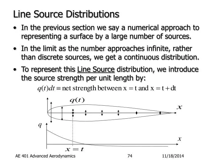
Line Source Distributions. In the previous section we say a numerical approach to representing a surface by a large number of sources. In the limit as the number approaches infinite, rather than discrete sources, we get a continuous distribution.

E N D
Line Source Distributions • In the previous section we say a numerical approach to representing a surface by a large number of sources. • In the limit as the number approaches infinite, rather than discrete sources, we get a continuous distribution. • To represent this Line Source distribution, we introduce the source strength per unit length by: AE 401 Advanced Aerodynamics
Line Source Distributions [2] • Rather than the summation we had for discrete sources, the total effect of a line source is found by integration. • Thus, for a line source running from leading to trailing edge of an airfoil, the stream and potential functions are: • These can still be combined with a uniform horizontal flow: AE 401 Advanced Aerodynamics
Thin Airfoil Theory – Symmetric • In Section 3.5 of the book, Moran discusses how to use these line distributions to model surfaces. • This is potentially a very complex task involving complex integrations. • However, some closed form mathematical solutions are possible if the Thin Airfoil assumptions are used. • To see this, first express the local velocities as the combination of the freestream plus local perturbations due to the line source: • Then our surface boundary condition is: AE 401 Advanced Aerodynamics
Thin Airfoil Theory – Symmetric [2] • However, if a body is very thin, then at most locations: • Thus, we can approximate the boundary condition by: • Similarly, the pressure coefficient given by: • Can be approximated by: AE 401 Advanced Aerodynamics
Thin Airfoil Theory – Symmetric [3] • These assumptions are obviously going to breakdown near the leading edge stagnation point where: • Not as obvious is the fact that they also breakdown at the trailing edge – where there is another stagnation point. • This aft stagnation point is obvious on cylinder, oval or ellipse shapes – but is much less pronounced on sharp trailing edge airfoils. • In real (i.e. viscous) flow, the boundary layer swallows this point within it, so it never really exists at all. AE 401 Advanced Aerodynamics
Thin Airfoil Theory – Symmetric [4] • Let’s for a moment ignore the problem at the stagnation points which we will revisit. • Instead, lets make one more approximation which takes a leap of faith. • Since we are considering only thin bodies, rather than apply the boundary condition on the surface, let’s apply it on the y=0 axis, or: • At first glance this might seem rediculous since we expect by symmetry that v=0 at y=0. • But, consider what a line source looks like. AE 401 Advanced Aerodynamics
Thin Airfoil Theory – Symmetric [5] • Since a source is spitting out mass, the vertical velocity jumps, or changes sign, across the line source. • Note also that there isn’t an infinite velocity on the line since there is not a radial change in flow area! • Since we are still only doing symmetric bodies, we only have to deal with one side right now – later, on lifting airfoils, we will have to deal with asymmetry. AE 401 Advanced Aerodynamics
Thin Airfoil Theory – Symmetric [6] • And, if we see how we are going to evaluate the local velocity due to the line source at y=0, we get: • While the numerator of the integrand will go to zero, realize that the denominator will go to zero also near where x=t. • Choose a small region around x=t, say from x- to x+ ( is very small), we can assume q(t) is constant in this interval and equal to q(x). • Everywhere else the integrand is zero. AE 401 Advanced Aerodynamics
Thin Airfoil Theory – Symmetric [7] • Thus: • When we combine this with the flow tangency boundary condition, we have a solution for q(x): AE 401 Advanced Aerodynamics
Thin Airfoil Theory – Symmetric [8] • To get the pressure distribution, we first need to evaluate the us velocity component, also at y=0: • The integrand in this equation has a singularity (goes to infinity) at x=t, if y is also equal to zero. • Dealing with this singularity require some complex math tricks. • The general idea is that this integral, unlike the previous one for vs, does not depend upon the value at x=t since the integrand is odd about that point (changes from positive to negative). AE 401 Advanced Aerodynamics
P P Thin Airfoil Theory – Symmetric [9] • Instead, the values of the integral upstream and downstream are what is important. • The way to express this integration which excludes a singularity, we use the Cauchy Principal Value integral. • After taking the limit and substiting the line strength as a function of surface slope, this becomes: AE 401 Advanced Aerodynamics
P Thin Airfoil Theory – Symmetric [10] • While this last equation does not seem to useful in integral form, for many possible functions for Y’, closed form solutions are possible using Appendix B. • So, to summarize, by thin airfoil theory on symmetric bodies: AE 401 Advanced Aerodynamics
Thin Airfoil Theory – Example 1 • To show how this analysis can work in practice, consider an elliptical airfoil whose surface is given by: • The thickness of this airfoil is t. Also, the surface slope is given by: • Thus, the source strengths are: AE 401 Advanced Aerodynamics
Thin Airfoil Theory – Example 1 [2] • Before attempting to integrate Y’(x) to find us, lets first introduce a change of variables which will make life easier: • The source distribution then becomes: AE 401 Advanced Aerodynamics
P Thin Airfoil Theory – Example 1 [3] • For the integration, we also need to change the dummy variable of integration to: • Finally, the limits of integration change since: • Thus, the integration becomes: • Which, using Appendix B, is just: • Note that this is a constant velocity! AE 401 Advanced Aerodynamics
Thin Airfoil Theory – Example 1 [4] • The pressure distribution is also constant: • The plot below show a comparison of this result to a numerical solution for the same shape: AE 401 Advanced Aerodynamics
surface line source Thin Airfoil Theory – Example 1 [5] • The plot shows that, surprisingly perhaps, thin airfoil does a good job of predicting the pressure distribution. • The error at the leading and trailing edge, the stagnation points, is understandable given the assumptions. • However, one way to explain the discrepancy is the fact that the source really shouldn’t extend to the leading edge: • If the line source started a little to the right of the y axis, a stagnation point would be formed. AE 401 Advanced Aerodynamics
surface line source r Thin Airfoil Theory – Example 1 [6] • Moran states the to model the leading edge, the source should be offset by an amount equal to half the leading edge radius, r. • In practice, we will just live with the error since the leading edge region is usually pretty small. AE 401 Advanced Aerodynamics
Thin Airfoil Theory – Example 2 • The second example Moran shows is for a very simple airfoil shape define by: • The solution in this case is: • This solution is compared to a numerical solution on the next slide. AE 401 Advanced Aerodynamics
Thin Airfoil Theory – Example 2 [2] • Once again, the match is pretty good, except for leading and trailing edges. • But, the complexity of the solution (and the math) has gone way up, and this is a very simple geometry. AE 401 Advanced Aerodynamics