Download
1 / 16
160 likes | 440 Views
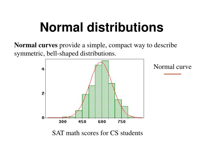
Normal distributions. Normal curves provide a simple, compact way to describe symmetric, bell-shaped distributions. . Normal curve. SAT math scores for CS students. Money spent in a supermarket. Is the normal curve a good approximation?. SAT math scores for CS students.

E N D
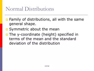
Normal distributions Normal curves provide a simple, compact way to describe symmetric, bell-shaped distributions. Normal curve SAT math scores for CS students
Money spent in a supermarket Is the normal curve a good approximation?
SAT math scores for CS students The area under the histogram, i.e. the percentages of the observations, can be approximated by the corresponding area under the normal curve. If the histogram is symmetric, we say that the data are approximately normal (or normally distributed). We need to know only the average and the standard deviation of the observations!!
SAT math scores for CS students The variable SAT math scores is normally distributed with Mean m= 595.28 and Std Deviation s = 86.40.
The standard normal curve The standard normal distribution has mean =0 and standard deviation =1 The curve is perfectly symmetric around 0 Any value on a normal curve can be converted to a value on the standard normal curve using this formula: (value – mean) / standard deviation
Graphing the normal curve using Excel Excel function NORMDIST = area under the normal curve Syntax NORMDIST(x, m, s, 1) = area to the left of x m=average & s=standard deviation NORMDIST(x, m, s, 0) = computes normal density function at x m=average & s=standard deviation Excel function NORMSDIST(x,1) = area under the standard normal curve (m=0, s=1)
Graphing the standard normal density curve • Open a new workbook • Enter the labels z and f(z) in cells A2 and B2 • Enter –3.5 & -3.4 in cells A3 and A4, click and drag down until you create the sequence of digits from –3.5 to 3.5. • Select B3 and enter =NORMDIST(A3,0,1,0) • Select B3 and drag down to B73 • Open the Chart Wizard, select XY (Scatter) • The data range should already be indicated.
Normal distribution function F(z) It is defined as the area under the standard normal to the left of z, that is F(z)=P(Z<=z)
Application of the normal distribution to the data Mean = 595.28 Std Dev. s = 86.40 The distribution of the SATM scores for the CS students is approximately normal with mean 595.28 and s.d. 86.40: N(595.28 , 86.40) Problem: What is the percentage of CS students that had SAT math scores between 600 and 750? Answer: Use the normal approximation - It is the area under the normal density curve between 600 and 750.
How do we compute it? We use the values of theNormal distribution function F(x)=P(X<=x). Problem: What is the percentage of CS students that had SAT math scores between 600 and 750? Approximate answer: The percentage of students with SATM between 600 and 750 is computed as 600 600 750 == __ 750 595.28 595.28 595.28
Using Excel • Select a cell, say A1 • Compute the area on the left of 600 as =NORMDIST(600, 595.28 , 86.40, 1). • Compute the area on the left of 750 as =NORMDIST(750, 595.28 , 86.40, 1). • The area under the curve between 600 and 750 is =NORMDIST(750, 595.28 , 86.40,1)- NORMDIST(600, 595.28 , 86.40, 600,1). • The answer is 0.44 – Approximately 44% of CS students in the survey have SATM between 600 and 750.
In summary • Follow the following steps: • State the problem. Calculate the sample average and the s.d. and define the interval you are interested in • Compute the area under the approximate normal density curve with mean and s.d. defined above.
Example Problem Problem: What is the lowest SAT math score that a student must have to be in the top 25% of all CS students in the sample? Mean = 595.28 Std Dev. s = 86.40 25% Sample Q3=650 ? Find the value x, such that 25% of observations fall at or above it.
Beware! Is the normal approximation appropriate for these data? Underestimate this area Overestimate this area Use it when the histogram of the observations is bell-shaped!