Distributions

1. Applied statistics for testing and evaluation – MED4 Distributions Lecturer: Smilen Dimitrov

2. Introduction • We previously discussed measures of • central tendency (location) of a data sample (collection) – arithmetic mean, median and mode; and • statistical dispersion (variability) – range, variance and standard deviation in descriptive statistics • Today we look into the concept of distributions in more detail, and introduce quantiles as final topic in descriptive statistics • We will look at how we perform these operations in R, and a bit more about plotting as well

3. Histogram view and standard errors • We already know how to calculate mean and standard deviation of a sample, and show a histogram (frequency count) of a data sample • Thus, we could write our results as: • “There are, on average, mean ± standard deviation raisins in a box” • “There are 27.95 ± 1.52 raisins in a box most of the time”

4. Histogram view and standard errors • The obtained numbers (mean) are an estimate based on only one data sample of 17 boxes • As we haven’t taken the entire population into account, they could be missed – also for the next sample they will be different – so estimate for mean value is unreliable • “There are 27.95 ± 1.52 raisins in a box most of the time” is an imprecise statement • We should provide a measure for unreliability, known as standard error.

5. Histogram view and standard errors • The obtained numbers are an estimate based on only one data sample of 17 boxes • Estimate for mean value is unreliable • We should provide a measure for unreliability, known as standard error. • So, we’d write “the mean of our sample is mean ± standard error (1 s.e., n=)”

6. mean value one standard error (above) one standard error (below) one standard deviation (above) one standard deviation (below) Histogram view and standard errors • “The mean number of raisins in our data sample was 27.95 ± 0.368 raisins per box (1 s.e., n=17) • Here we are trying to infer an estimate about the population based on the sample. • 'What can I say about a whole population based on information from a random sample of that population?' • 'To what degree can I say that my estimate is accurate?' • To proceed with inferential statistics, we need to introduce concept of distributions.

7. mean value one standard error (above) one standard error (below) one standard deviation (above) one standard deviation (below) Histogram view and standard errors • “The mean number of raisins in our data sample was 27.95 ± 0.368 raisins per box (1 s.e., n=17) • The standard deviation (SD) describes the variability between individuals in a sample; • the standard error of the mean (SEM) describes the uncertainty of how the sample mean represents the population mean. • Authors often, inappropriately, report the SEM when describing the sample. As the SEM is always less than the SD, it misleads the reader into underestimating the variability between individuals within the study sample.

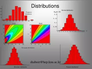
8. Distributions - frequency and probability • Distribution – which mathematical function can be used to approximate a histogram (frequency count) • Frequency distribution - a list of the values that a variable takes in a data sample - and how many times they occur, expressed as relative frequencies. • Refers to a particular data sample, like the particular 17 boxes of raisins in our example. So far, the histogram of the sample we’ve drawn is a frequency distribution. • Statistical hypothesis testing is founded on the assessment of differences and similarities between frequency distributions. This assessment involves measures of central tendency or averages, such as the mean and median, and measures of variability or statistical dispersion, such as the standard deviation or variance. • Probability distributions – idealized mathematical functions, that result with probabilities – predictions / estimates about unknown (future) values of a variable.

9. Distributions - frequency and probability • Based on a frequency distribution, we try to determine the probability distribution of the underlying process, so we could estimate/predict changes of the variable. • In statistics, we use mathematical probabilities to predict the expected frequencies of outcomes from repeated trials of random experiments. • If we repeat the random experiment over and over and summarize the results, a pattern of outcomes begins to emerge. • We can determine this pattern by repeating the experiment many, many times, or we can also use mathematical probabilities to describe the pattern. Probability distribution Frequency distribution

10. Probability • The theory of probability attempts to quantify the notion of probable. • just as the theory of mechanics assigns precise definitions to such everyday terms as work and force. • probable is one of several words applied to uncertain events or knowledge, being closely related in meaning to likely, risky, hazardous, and doubtful. • In an experiment of a coin toss, we want to quantify how probable it is that the next toss will be, say, heads. • A subject repeatedly attempts a task with a known probability of success due to chance, then the number of actual successes is compared to the chance expectation (probability). • If a subject scores consistently higher or lower than the chance expectation after a large number of attempts, one can calculate the probability of such a score due purely to chance, and then • argue, if the chance probability is sufficiently small, that the results are evidence for the existence of some mechanism (precognition, telepathy, psychokinesis, cheating, etc.) which allowed the subject to perform better than chance would seem to permit.

11. Probability • Predictable phenomena (tossing a coin) • Aleatory probability, which represents the likelihood of future events whose occurrence is governed by some random physical phenomenon. • Unpredictable phenomena (radioactive decay) • Epistemic probability, which represents one's uncertainty about propositions when one lacks complete knowledge of causative circumstances. (to determine how 'probable' it is that a suspect committed a crime, based on the evidence presented.) • Question of probability interpretations - what can be assigned probability, and how the numbers so assigned can be used. • Bayesian interpretation - there are some who claim that probability can be assigned to any kind of an uncertain logical proposition. • Frequentist interpretation - there are others who argue that probability is properly applied only to random events as outcomes of some specified random experiment, for example sampling from a population.

12. Probability • The probability of an event is generally represented as a real number (p) between 0 and 1, inclusive. • An impossible event has a probability of exactly 0, and a certain event has a probability of 1 (but the converses are not always true) • Most probabilities that occur in practice are numbers between 0 and 1, indicating the event's position on the continuum between impossibility and certainty. The closer an event's probability is to 1, the more likely it is to occur. • For example, if two mutually exclusive events are assumed equally probable, such as a flipped or spun coin landing heads-up or tails-up, we can express the probability of each event as '1 in 2', or, equivalently, '50%' or '1/2'. • Odds a:b for some event are equivalent to probability a/(a+b).

13. Probability • Formal laws of probability can be expressed as: • a probability is a number between 0 and 1 (0 ≤ p ≤ 1) • the probability of an event or proposition and its complement must add up to 1 ( ); • the joint probability of two events or propositions is the product of the probability of one of them and the probability of the second, conditional on the first. • Mathematical meaning: - If we repeat the random experiment, a pattern of outcomes begins to emerge. We can use mathematical probabilities to describe the pattern. • by saying that 'the probability of heads is 1/2', we mean that, if we flip our coin often enough, eventually the number of heads over the number of total flips will become arbitrarily close to 1/2; and will then stay at least as close to 1/2 for as long as we keep performing additional coin flips.

14. Probability distributions • Laplace (1774) - law of probability of errors by a curve y = f(x), x being any error and y its probability, and laid down three properties of this curve: • it is symmetric as to the y-axis; • the x-axis is an asymptote, the probability of the error ∞ being 0; • the area enclosed is 1, it being certain that an error exists. • Every random variable gives rise to a probability distribution, and this distribution contains most of the important information about the variable. • A probability distribution is a function that assigns probabilities to events or propositions. • (alt) A probability distribution function, assigns to every interval of the real numbers a probability, so that the probability axioms are satisfied. • For any set of events or propositions there are many ways to assign probabilities, so the choice of one distribution or another is equivalent to making different assumptions about the events or propositions in question.

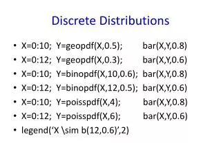
15. Probability distributions • Discrete distribution - if it is defined on a countable, discrete set, such as a subset of the integers. • Continuous distribution - if it has a continuous distribution function, such as a polynomial or exponential function. • Equivalent ways to specify a probability distribution: • The most common is to specify a probability density function (pdf). Then the probability of an event or proposition is obtained by integrating the density function. • The distribution function may also be specified directly. In one dimension, the distribution function is called the cumulative distribution function (cdf).

16. Probability distributions – CDF and PDF • If X is a random variable, the corresponding probability distribution assigns to the interval [a, b] the probability Pr[a ≤ X ≤ b], i.e. the probability that the variable X will take a value in the interval [a, b]. • The probability distribution of the variable X can be uniquely described by its cumulative distribution function F(x), which is defined by for any x in R. • The distribution function F(x), also denoted D(x) (also called the cumulative density function (CDF) or probability distribution function), describes the probability that a variate X takes on a value less than or equal to a number x. • The probability function P(x) (also called the probability density function (PDF) or density function) of a continuous distribution is defined as the derivative of the cumulative distribution function F(x).

17. Uniform distribution • Discrete uniform distribution - characterized by saying that all values of a finite set of possible values are equally probable • If a random variable has any of n possible values k1, k2, …, kn that are equally probable, then it has a discrete uniform distribution. The probability of any outcome ki is 1/n. Probability Distribution applet Probability (applet)

18. Uniform distribution continuous discrete

19. Normal (Gaussian) distribution • The normal distribution, also called Gaussian distribution, is an extremely important probability distribution in many fields. • It is a family of distributions of the same general form, differing in their location and scale parameters: the mean ('average') and standard deviation ('variability'), respectively. • The standard normal distribution is the normal distribution with a mean of zero and a standard deviation of one. It is often called the bell curve. • The fundamental importance of the normal distribution as a model of quantitative phenomena in the natural and behavioral sciences is due to the central limit theorem (the proof of which requires rather advanced undergraduate mathematics). • A variety of psychological test scores and physical phenomena like photon counts can be well approximated by a normal distribution. • While the mechanisms underlying these phenomena are often unknown, the use of the normal model can be theoretically justified if one assumesmany small (independent) effects contribute to each observation in an additive fashion. U of T Day Statistics Applets

20. Normal (Gaussian) distribution continuous discrete • The discrete version is known as binomial distribution. (The probability of making a certain number of correct guesses of coin toss/dice by chance.) • The pdf can be expressed analytically, but the cdf (that is, the error function) cannot (so it must be computed numerically) • The cdf can be understood as area under the pdf curve. Cannot be expressed analytically Normal Distribution applet

21. Normal (Gaussian) distribution • The normal distribution can give a lot of information based on its shape (scores)

22. Central limit theorem • The central limit theorem states that: • the mean of any set of variates with any distribution having a finite mean and variance tends to the normal distribution; or • if the sum of the variables has a finite variance, then it will be approximately normally distributed. • Addition and subtraction of variates from two independent normal distributions with arbitrary means and variances, are also normal! • Since many real processes yield distributions with finite variance, this explains the ubiquity of the normal distribution. • Many common attributes such as test scores, height, etc., follow roughly normal distributions, with few members at the high and low ends and many in the middle.

23. Central limit theorem illustration • Concrete illustration - suppose the probability distribution of a random variable X puts equal weights on 1, 2, and 3. • Now consider the sum of two independent copies of X.

24. Central limit theorem illustration • Now consider the sum of three independent copies of this random variable.

25. Central limit theorem illustration • Applets: Central Limit Theorem Demo Applet (22-Jul-1996) The Central Limit Theorem (applet) Introduction To Probability Models Central Limit Theorem Explained Probability Distribution Central Limit Theorem

26. R example • Fitting a normal distribution to our raisin data sample

27. Quantiles • Quantiles are essentially points taken at regular intervals from the cumulative distribution function (cdf) of a random variable. • Dividing ordered data into q essentially equal-sized data subsets is the motivation for q-quantiles; the quantiles are the data values marking the boundaries between consecutive subsets. • Quantiles are dependent on the assumed distribution – here shown for the normal distribution • Some quantiles have special names: • The 100-quantiles are called percentiles. • The 10-quantiles are called deciles. • The 5-quantiles are call quintiles. • The 4-quantiles are called quartiles.

28. Quantiles – data samples • For data samples, we can work without knowing the distribution. For example, given the 10 data values {3, 6, 7, 8, 8, 10, 13, 15, 16, 20}, the first quartile is determined by 10*1/4 = 2.5, which rounds up to 3, and the third sample is 7. • The second quartile value (same as the median) is determined by 10*2/4 = 5, which is an integer, so take the average of the fifth and sixth values, that is (8+10)/2 =9, though any value from 8 through to 10 could be taken to be the median. • The third quartile value is determined by 10*3/4 = 7.5, which rounds up to 8, and the eighth sample is15. • The motivation for this method is that the first quartile should divide the data between the bottom quarter and top three-quarters. Ideally, this would mean 2.5 of the samples are below the first quartile and 7.5 are above. • Notice, for this data sample, helps us tell that it is not normally distributed!

29. A simple normality test • A normal distribution will have 95 % of the values occuring between –1.96 to 1.96 standard deviations around the mean, 2.5% lie above, and 2.5% lie below. • A simple normality test is to check whether this holds for a given data sample. • If this is not the case, then our samples are not normally distributed.They might for instance, follow a Students' t distribution. 95 % range • Student's t distribution is used instead of the Normal distribution when sample sizes are small (n<30).

30. Max value 3rd quartile (75%) Interquartile range Median = 2nd quartile (50%) Range 1st quartile (25%) Min value Statistics summary and 'box and whisker' plots • Statistics summary for a data collection – mean, median, range, standard deviation, quantiles • A visualization of this summary is a box (and whisker) plot

31. Review • Arithmetic mean • Median • Mode • Range • Variance • Standard deviation • Quantiles, • Interquartile range • Probability distributions – uniform and normal (Gaussian) • Standard error – inference about unreliability Measures of Central tendency (location) Descriptive statistics Measure of Statistical variability (dispersion - spread) Inferential statistics

32. Exercise for mini-module 4 – STAT04 Exercise 1. Import the data into R, and for each garden, summarize the data (mean, median, variance, standard deviation, interquartile range). 2. Using R, visualise the summaries for each garden as a box plot. Arrange the box plots one after another horizontally on the same graph. Make sure that corresponding axes are matching, to allow for visual comparison. 3. Using R, plot the relative frequency histogram for each of the gardens. Arrange these plots one after another vertically on the same graph. Make sure that corresponding axes are matching, to allow for visual comparison. Fit each histogram with its corresponding normal distribution. 4. Plot the 95% probability range of the normal distribution for each garden on the plots from (3). Which of these data samples (if any) can be seen as being normally distributed and why? Delivery: Deliver the collected data (in tabular format), the found statistics and the requested graphs for the assigned years in an electronic document. You are welcome to include R code as well. Use the following data: The data in the following table come from three garden markets. The data show the ozone concentrations in parts per hundred million (pphm) on ten consecutive summer days