Download
1 / 32
320 likes | 328 Views
Time-of-Flight at CDF. Matthew Jones August 19, 2004. History. An experimental TOF system installed in CDF at the end of Run-I: Covered only 5% of the acceptance Demonstrated feasibility Identified potential problems Contributions to Run-II TOF system from several institutes:

E N D
Time-of-Flight at CDF Matthew Jones August 19, 2004
History • An experimental TOF system installed in CDF at the end of Run-I: • Covered only 5% of the acceptance • Demonstrated feasibility • Identified potential problems • Contributions to Run-II TOF system from several institutes: • Cantabria, FNAL, INFN, Korea, LBL, MIT, Penn, Tsukuba
Introduction • Tracking chambers only detect stable, charged particles: • PT measured by curvature in B field • Extra information needed for particle ID: • Ionization of material • Cherenkov techniques • Time-of-Flight • Shower shapes • Transition radiation These measure e/h separation
Measuring t Detector Production point • How well we can measure t determines how well we can distinguish between the two particles.
Time-of-Flight • Achievable resolution is of order 100 ps.
Measuring TOF • Important issues: • Precision: K/ separation or cosmic veto? • Detector technology: • Scintillator + PMT • Resistive plate chambers • Segmentation: occupancy vs channel count • Cost per channel
Detecting charged particles • Charged particles lose energy in material: • Example: 1 MIP = 2 MeV/cm
Plastic Scintillator • Ionization excited molecular states • electrons are loosely bound • Ionization excites the S0 electrons • Light emitted when de-excitation occurs • Emission spectra shifted to lower energies • Absorption and emission spectra do not overlap emitted light is not re-absorbed.
Properties of Plastic Scintillator • Typical figures of merit: • Light yield (% compared with anthracene) • Emission spectrum • Bulk attenuation length • Rise time, decay times (short, long) • Bicron-408: • r = 0.9 ns, f = 2.1 ns • Bulk attenuation length, = 380 cm
Examples from Bicron Blue
Photomultiplier Tubes • Books from vendors are fun to read:
Photomultiplier Tubes • Mesh dynode structure: • This kind will work in a magnetic field. • Typical construction: • This kind won’t work in a magnetic field.
Photomultiplier Tubes • Window material: • Borosilicate glass: transmits blue (not UV) • Photocathode: • Bialkali metal (Sb-Rb-Cs): low work function • Also important: low dark current • Dynodes: • Metal with secondary emissive material • Good (relatively inexpensive): Be-CuO-Cs • Better (more expensive): GaP: Cs
Photomultiplier Tube Properties • Quantum efficiency: 20% at 390 nm • Gain: • With n=19, ~ 107 at 2 kV and no B field • Gain greatly reduced in a magnetic field 2R ~2 kV
Mesh PMT’s in Magnetic Fields • Gain is reduced by ,but not to zero • Large tube-to-tube variation 1.4 Tesla
Preamp for PMT • We added a preamplifier with a gain of 15 • Differential output driver • Gain switches to ~2 for big pulses preamp
Photomultiplier tube properties • Timing characteristics: • Pulse shape: Gaussian, few ns risetime • Transit time: ~ 15 ns • Transit time spread: ~ 300 ps Timing resolution is roughly TTS / √n That’s why we want n to be large.
Photomultiplier tube properties Gain Transit time Pulse rise time Pulse width
PMT-Scintillator interface • Scintillator dimensions is about 2x2 cm • Sensitive area of photocathode is 27 mm • Optical couplings made using glue or silicone pads
The CDF-II TOF System Look for it here…
The CDF-II TOF System The PMT goes in here.
Front-end Electronics • Requirements: • Measure arrival time of pulse from PMT • Measure pulse height (or charge) • Do it every 132 ns (whimsical requirement) • Precision should be < 25 ps • Limitations: • Only measures time of first pulse • Light from multiple pulses overlap (biases Q)
Front-end Electronics • Fast components go to discriminator. • Slow components used to measure charge. High pass filter Low pass filter
Measuring Time • Time measured using TAC with respect to a common stop signal: Voltage proportional to time difference between START and STOP
Interface with ADMEM • Use ADMEM boards to read out TOF: • CAFÉ cards measure charge • deCAF cards measure time (output of TAC) TOMAIN ADMEM deCAF CAFE TOAD 9 channels TOAD TOAD
Typical Response • Response of PMT from cosmic rays: 132 ns
Pulse Properties • Pulse shape is a complicated mixture of • Scintillation process • Light transport in the scintillator • Optics of PMT coupling • PMT response • Shaping from base • Preamplifier • Cables • Receiver and discriminator
Things we can’t measure directly • Absolute gain: • Need calibrated light source (we do have a laser…) • Need magnetic field • Systematics from electronics (preamp,QanodeADC?) • Probably averages around 3 x 10⁴ • Number of photons: • Don’t know PMT properties well enough • Don’t know the gain precisely • Systematics from electronics • Probably end up with few 100 p.e. • Most effects are parameterized by the empirical model used for calibration.
Simulated pulses • We can’t probe the electronics on CDF to see what the pulses really look like. • Simulations can provide a qualitative description of most effects. Scintillator bar Far PMT Muon Near PMT
Simulated pulses • Compare pulse shapes at east/west ends: Attenuated far pulse
Timing Resolution • Stated goal was “100 ps”. • Actual model is: • Resolutions measured after calibrations: • Not the complete story, see next talk by Stephanie…
Summary • Typical TOF detector • BC-408 scintillator • Mesh PMT’s • Properties poorly controlled – each channel is different • Unique features • Hadron collider environment • Small bar cross section: not much light output • DAQ interface • Looks like one of the calorimeters • Performance • Generally meets timing precision requirements…