Download
1 / 39
390 likes | 404 Views
Gaseous time-of-flight detectors. P.Fonte. Outlook The timing RPC Detector physics avalanche physics time resolution number of gas gaps choice of gas gap width importance of space-charge Readout issues Signal and electronics Pads vs. strips Crosstalk Conclusion.

E N D
Gaseous time-of-flight detectors P.Fonte
Outlook • The timing RPC • Detector physics • avalanche physics • time resolution • number of gas gaps • choice of gas gap width • importance of space-charge • Readout issues • Signal and electronics • Pads vs. strips • Crosstalk • Conclusion
The timing RPC detector technology -HV Particle E Resistive material, glass Sensitive Area Conductive material, Aluminum • Main features • Timing resolution ~ 50 ps σ. • Efficiency 75% for a 300 μm gap • No energy resolution. • Possibility to measure the position. • No sparking (only small local discharges called “streamers”) Precise gas gap with few 100 mm MIPS Gas gap
HV Main timing RPC applications (since 2000) All practical tRPCs in operation are “multigap” [ Williams 1996] and symmetric, use a gas mixture composed of C2H2F4, SF6 and eventually C4H10 in various proportions. Except HARP, all detectors show a time resolution between 40 and 80 ps and efficiency >97% (details may depend also on the measurement setup). symmetric multigap RPC Timing RPC: a revolution in TOF technology for High-Energy and Nuclear physics
Detector physics 2 main questions: 1-How is it possible to reach 50 ps resolution in a gas counter? 2-How is it possible to reach efficiencies of 75% in a 0.3 mm gas gap? Enormous space-charge effect
Time resolution-basics i cathode anode i Detection level independent from the cluster position exact timing (If no primary statistics or avalanche statistics)
Time resolution-basics i cathode Time needed to reach agiven current depends on avalanche growth statistics (exponential distribution). Several clusters (Poisson distribution) anode i [Werner Riegler, Elba, 2003] Detection level independent from the cluster position exact timing (If no primary statistics or avalanche statistics)
Time resolution-basics i cathode Time needed to reach agiven current depends on avalanche growth statistics (exponential distribution). Several clusters (Poisson distribution) anode i i0
Time resolution-basics analytical model i cathode Time needed to reach agiven current depends on avalanche growth statistics (exponential distribution). Several clusters (Poisson distribution) anode i i0 [Mangiarotti, Fonte and Gobbi, RPC2003] Detection level independent from the cluster position exact timing (If no primary statistics or avalanche statistics)
Time resolution - analytical model Single-cluster Basic time scale: ~100 ps. The i0 distribution is translated into a time distribution by action of the discriminating level. Slope=*vd [Mangiarotti, Fonte and Gobbi, RPC2003] i0 • The time resolution depends essentially only on 2 parameters: • -linearly on 1/(*vd) = average time between ionizing colisions • -on the average number of effective clusters (r n0)
Time resolution - analytical model • Universal curves • The resolution is a function of the ineficiency only • Asymptotic 1/(N) behaviour Observable resolution should be somewhat better, as the time somewhat intrinsically correlateswith charge (on top of the trivial electronics risetime effect) and can be corrected.
Example: 2D-position sensitive readout Time signal HV X right X left XY readout plane out left 4 cm 10 strips for each coordinate at 4 mm pitch Y-strips (on PCB) out right RC passive network RC passive network X-strips (deposited on glass) Precise construction 2 mm thick black glass lapped to ~1m flatness metal box (no crosstalk) 300 m thick high glass disk (corners) Well carved into the glass (avoid dark currents from the spacer) [Blanco 2002] Resistive division (for small and accurate TOF systems)
Example: 2D - position-sensitive Y(mm) Events/mm2 X (mm) 1500 Trigger edge (3 mm) Chamberedge 1000 Events/0.5mm 500 0 -25 -20 -15 -10 -5 0 5 10 15 20 25 Position along X (mm) 1500 2 2 10 10 4 mm strip pitch 1000 Events/0.5mm Events/4ps Events/4ps 1 1 10 10 500 0 0 0 10 10 10 15 20 -25 -20 -15 -10 -5 0 5 25 -1000 -500 0 500 1000 -1000 -500 0 500 1000 Position along Y (mm) Time difference (ps) Time difference (ps) Position resolution (=75%) No edge effects edges 3 mm resolution 3 mm FWHM (strips=4mm) Edge & Corner Sigma=76.9 ps (66 ps) Center Sigma=74.0 ps (62 ps) [Blanco 2002]
Example: Small single counters (9 cm2) -HV 3 4 x 0.3 mm gaps [ Fonte 2000] Aluminum Glass Resolution of thereference counter • = 99.5 % for MIPs (75%/gap) (optimum operating point 1% of discharges)
Example: 24 gap multigap RPC [S.An, 2008] Single-point measurement between identical counters. All systematic errors cancel out.
What is the real advantage of many gas gaps? • More efficiency: YES. 1-(1-0.75)N (single gap=75%) • Better timing: YES. ~1/N • Larger signal? • Better charge spectra?
Induced signal strenght vs. geometric dimensions i(t) Q3(t) Q2(t) d Q1(t) g No real advantage in having many or wider gaps qind = fast (electronic) induced charge: the useful signal Ewis the “weighting field”, which accounts for the coupling (electrical induction) between the avalanche charges and the electrodes 1/ln(G) is related to the details of the avalanche development. This is a complex matter, but experimentally a value of 1/10 is often found g is the gap width d is the glass thickness For a regular structure (all d’s and g’s the same) r =relative permittivity of the glass ~4
Charge spectra 4-fold convolution of a single-gap spectrumsuperimposed on the measured 4-gap spectrum Measured single-gap fast (electronic component) charge spectrum [Fonte 1999] 4-fold convolution measured 10-gap spectrum Space-charge gain limit [Akindinov et al. 2004] N-fold convolution gaussian
What is the real advantage of many gas gaps? • More efficiency: YES. 1-(1-0.75)N (single gap=75%) • Better timing: YES. ~1/N • Larger signal: NO. The increase in the generated charge is compensated by the larger distance to the readout electrodes • Better charge spectra: YES. Tends to gaussian.
Single-cluster Basic time scale: ~100 ps. theoretical ~1/Q Space-charge effect What gas gap width? • The higher the gain the better because the ionization rate v sets the time scale • Limitation: too many streamers • Smaller gaps require higher v for thesame gain (favourable) • Furthermore, in a small gap a large v results on a comparatively small avalanche owing to the space-charge effect, avoiding disturbing streamers. (Very hard effect to calculate.) • Empirical optimum 200 to 300 µm
Electrode shape time jitter Distribution of position-time jitter • PADS: • 2n geometry (ALICE TOF) • HARP (analog sum) Impact on gaussian resolution Usable up to ~100 mm wide pads • Possible further problem: • large geometrical and impedance mismatch may lead to excessive signal loss
Electrode shape STRIPS: introduced in the famous Pestov counter • Solves the problem because: • average time (between ends) is independent from the particle position (TOF) • difference time is independent from TOF and gives the particle position
Example: Large tRPC counter 1,6 m HV 4 timing channels Ordinary 3 mm “window glass” 5 cm Copper strips Active area = 10 cm160 cm = 0.16 m2(400 cm2/electronic channel) Top view Cross section [Blanco 2001]
Example: Large tRPC counter 100% = 95 to 98 % 99% 98% 97% Time efficiency 96% Strip A 95% Strip B 94% Strips A+B 93% -80 -70 -60 -50 -40 -30 -20 -10 0 10 20 30 40 50 60 70 80 Center of the trigger region along the strips (cm) 100 = 50 to 75 ps 90 80 Time resolution (ps ) 70 60 50 40 -80 -70 -60 -50 -40 -30 -20 -10 0 10 20 30 40 50 60 70 80 Center of the trigger region along the strips (cm) Efficiency and time resolution [Blanco 2001] No degradation when the area/channel was doubled (800 cm2/channel)
Example: FOPI’s multistrip multigap (MMRPC) [M.Kis, CBM coll. meeting 2008] 16 strips, exactly 50 impedance, readout from both sides
Example: FOPI’s multistrip multigap (MMRPC) [Schuetauff, 2006] Unfortunately, no multihit data has been published
Strips: the crosstalk problem In a multiconductor transmission line (MTL) the electrodes couple via mutual capacitance and inductance. Exact theory exists. Good match with measurements. Crosstalk amplitude in 2-strips approximation [Gonzalez-Diaz 2011] Inducto-capacitivecoupling Modal-dispersioncoupling Depends essencially on the self and mutual capacities (Cm, Cg) and on the same with the dielectrics removed (Cm0, Cg0).
Strips: the crosstalk problem Cm=88 pF/m BW=1.5 GHz Rin=50 Ω Zc~13 Ω Cg=514 pF/m 1,6 m 5 cm Cm/Cg =17% Fct=50%! very dispersive! transverse scan 'fine-tunning' Fct=40% Data [Blanco 2001] Calculation [Gonzalez-Diaz, talk at IEEE NSS 2009] 80%-90% measured cross-talk levels reproduced
Recent results on crosstalk for CBM@GSI ... ... [Wang et al., IEEE NSS 2010] Observable crosstalk is only a few % except for large charge (streamers)
Recent results on crosstalk for CBM@GSI [I.Deppner,etal., in pressdoi:10.1016/j.nima.2010.09.165] Total observable crosstalk is only 2-3%.
Example: shielded tRPCs for HADES@GSI Further shielding between feedthrougs 1200 individually-shielded monostrip counters
Example: shielded tRPCs for HADES@GSI Full area measurement between identical counters. Some systematic errors may cancel.
Example: shielded tRPCs for HADES@GSI Despite extensive shielding a residual 20 ps “subtle” crosstalk effect remains No other multihit time resolution measurement is available in the literature
Multihit resolution calculation [Gonzalez-Diaz, talk at IEEE NSS 2009] (typical 1/20!...)
Multihit resolution calculation ... ... [Gonzalez-Diaz, talk at IEEE NSS 2009]
Conclusion • Timing RPCs are now the standard technique for TOF measurements in HEP and Nuclear Physics • Massive applications, previously impossible, were deployed and others are under study • Resolutions from 40 to 80 ps are easily reached with efficiency > 98%. • Pad readout is limited to ~10 cm wide pads owing to timing and maybe electrical limitations • Shielded monostrip readout has been shown to provide robust multihit performance at the expense of more complex mechanics • Multistrip detectors were deployed and are being further developed but their multihit time resolution in remains unproven