Download
1 / 15
330 likes | 1.77k Views
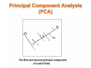
Principal Component Analysis (PCA). Dated back to Pearson (1901) A set of data are summarized as a linear combination of an ortonormal set of vectors which define a new coordinate system. Figure from Hastie, et, al 2001. Principal Components Analysis (PCA). Principal Components Analysis (PCA).

E N D
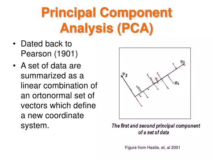
Principal Component Analysis (PCA) • Dated back to Pearson (1901) • A set of data are summarized as a linear combination of an ortonormal set of vectors which define a new coordinate system. Figure from Hastie, et, al 2001
Example 1 • Use the data set "noisy.mat" available on the course web page. The data set consists of 1965, 20-pixel-by-28-pixel grey-scale images distorted by adding Gaussian noises to each pixel with s=25.
Example 1 • Apply PCA to the noisy data. Suppose the intrinsic dimensionality of the data is 10. Compute reconstructed images using the top d = 10 eigenvectors and plot original and reconstructed images
Example 1 • If original images are stored in matrix X (it is 560 by 1965 matrix) and reconstructed images are in matrix X_hat , you can type in • colormap gray and then • imagesc(reshape(X(:,10),2028)’) • imagesc(reshape(X_hat(:,10),2028)’) to plot the 10th original image and its reconstruction.
Example 2 • Load the sample data, which includes digits 2 and 3 of 64 measurements on a sample of 400. load 2_3.mat • Extract appropriate features by PCA [u s v]=svd(X','econ'); • Create data Low_dimensional_data=u(:,1:2); • Observe low dimensional data Imagesc(Low_dimensional_data)