Download
1 / 23
230 likes | 379 Views
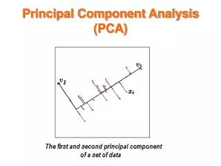
Principal Component Analysis (PCA). Principal Component Analysis (PCA). Principal Component Analysis (PCA). Principal Component Analysis (PCA). Principal Component Analysis (PCA). Principal Component Analysis (PCA). Principal Component Analysis (PCA). Principal Component Analysis (PCA).

E N D
Example 1 • Use the data set "noisy.mat" available on your CD. The data set consists of 1965, 20-pixel-by-28-pixel grey-scale images distorted by adding Gaussian noises to each pixel with s=25.
Example 1 • Apply PCA to the noisy data. Suppose the intrinsic dimensionality of the data is 10. Compute reconstructed images using the top d = 10 eigenvectors and plot original and reconstructed images
Example 1 • If original images are stored in matrix X (it is 560 by 1965 matrix) and reconstructed images are in matrix X_hat , you can type in • colormap gray and then • imagesc(reshape(X(:,10),2028)’) • imagesc(reshape(X_hat(:,10),2028)’) to plot the 10th original image and its reconstruction.
Example 2 • Load the sample data, which includes digits 2 and 3 of 64 measurements on a sample of 400. load 2_3.mat • Extract appropriate features by PCA [u s v]=svd(X','econ'); • Create data Low_dimensional_data=u(:,1:2); • Observe low dimensional data Imagesc(Low_dimensional_data)