Principal component analysis (PCA)

1. Principal component analysis (PCA) • Purpose of PCA • Covariance and correlation matrices • PCA using eigenvalues • PCA using singular value decompositions • Selection of variables • Biplots • References

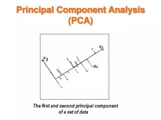
2. Purpose of PCA The main idea behind the principal component analysis is to represent multidimensional data with fewer number of variables retaining main features of the data. It is inevitable that by reducing dimensionality some features of the data will be lost. It is hoped that these lost features are comparable with the “noise” and they do not tell much about underlying population. The method PCA tries to project multidimensional data to a lower dimensional space retaining as much as possible variability of the data. This technique is widely used in many areas of applied statistics. It is natural since interpretation and visualisation in a fewer dimensional space is easier than in many dimensional space. Especially if we can reduce dimensionality to two or three then we can use various plots and try to find structure in the data. Principal components can also be used as a part of other analysis. Its simplicity makes it very popular. But care should be taken in applications. First it should be analysed if this technique can be applied. For example if data are circular then it might not be wise to use PCA. Then transformation of the data might be necessary before applying PCA. PCA is one of the techniques used for dimensional reductions.

3. Covariance and Correlation matrices Suppose we have nxp data matrix X: Where rows represent observation number and columns represent variable number. Without loss of generality we will assume that column totals are 0. If it would not be case then we could calculate column averages and subtract from each column this average. Covariance matrix is calculated using (it is true if column averages are 0): Correlation matrix is calculated using: I.e. by normalisation of covariance matrix by its diagonals. Both these matrices are symmetric and non-negative definite.

4. PCA using eigenvalues We have variable in p dimensional space. We want to find new variable (say a) that will have largest variation. Mathematically it can be written as: But by multiplying to a scalar value this expression (quadratic form) can be made as large as desired. Then we require that length of the vector is unit. I.e. vector satisfies the condition: Now if we use Lagrange multipliers technique then it reduces to unconditional maximisation of: If we get derivative of the left side and equate to 0 we have: Thus the problem of finding unit length vector with largest variance reduces to finding the largest eigenvalue and corresponding eogenvector. If we have largest eigenvalue and corresponding eigenvector then we can find second largest eigenvalue and so on. Finding principal components reduces to finding all egienvalues and eigenvectors of the matrix S.

5. PCA and eigenvalues Note that since matrix S is symmetric and non-negative definite all eigenvalues are non-negative and eigenvectors are orthonormal. I.e.: ai-s are known as the principal components. var(aix)=i. First principal component accounts the largest amount of the variance in the data. Elements of the vector ai contains coefficients of the ith principal component. Xai gives scores of the n individuals (observation vectors) on this principal component. Relation: shows that sum of the eigenvalues is equal to the total variance in the data. If instead of the covariance the correlation matrix is used then this sum is equal to the dimension of the original variable – p. Variance of i-th principal component is i. It is often said that this components accounts i/j proportion of the total variance. Plotting the first few principal components may show some structure in the data.

6. PCA using SVD Since we know that principal component analysis is related with eigenvalue analysis we can use similar techniques available in linear algebra. Suppose that X is mean centered data matrix. Then we can avoid calculating covariance matrix by using singular value decomposition. If we have the matrix nxp we can use SVD: where U is nxnV is pxp orthogonal matrices. D is nxp matrix. p diagonal elements contains square root of the eigenvalues of XTX and all other elements are 0. Rows of V contains coefficients of the principal components. UD contains scores of the principal components. Some statistical packages use eigenvalues for principal component analysis and some use SVD. Another way of applying SVD is using decomposition: Where U is nxp matrix  is pxp diagonal singular values matrix containing square roots of the eigenvalues of XTX and V is pxp orthogonal matrix that contains principal components. This decomposition is used for bi-plots to visualise data in an attempt to find structure in them.

7. Scaling It is often the case that different variables have completely different scaling. For examples one of the variables may have been measured in meters and another one in centimeters (by design or accident). Eigenvalues of the matrix is scale dependent. If we would multiply one column of the data matrix X by some scale factor (say s) then variance of this variable would increase by s2 and this variable can dominate whole covariance matrix and hence whole eigenvalue and eigenvectors. It is necessary to take precautions when dealing with the data. If it is possible to bring all data to the same scale using some underlying physical properties then it should be done. If scale of the data is unknown then it is better to use correlation matrix instead of the covariance matrix. It is in general recommended option in many statistical packages. It should be noted that since scale affects eigenvalues and eigenvectors then interpretation of the principal components derived by these two methods can be completely different. In real life application care should be taken when using correlation matrix. Outliers in the observation can affect covariance and hence correlation matrix. It is recommended to use robust estimation for covariances (in a simple case by rejecting of outliers). When using robust estimates covariance matrix may not be non-negative and some eigenvalues might be negative. In many applications it is not important since we are interested in the principal components corresponding to the largest eigenvalues. Standard packages allow using covariance as well as correlation matrices. R allows to input the correlation or the coavariance matrices also.

8. Screeplot Scree plot is the plot of the eigenvalues against their indices. For example plot given by R. When you see this type of plot with one dominant eigenvalue (variance) then you should consider scaling.

9. Dimension selection There are many recommendations for the selection of dimension. Few of them are: • The proportion of variances. If the first two components account for 90% or more of the total variance then further components might be irrelevant (Problem with scaling) • Components below certain level can be rejected. If components have been calculated using correlation matrix often those components with variance less than 1 are rejected. It might be dangerous. Especially if one variable is independent of the others then it might give rise the component with variance less than 1. It does not mean that it is uninformative • If accuracy of the observations is known then components with variances less than observations certainly can be rejected. • Scree plot. If scree plots show elbow then components with variances less than this elbow can be rejected. • There is cross-validation technique. One value of the observation is removed (xij) then using principal components this value is predicted and it is done for all data points. If adding the component does not improve prediction power then this component can be rejected. This technique is computer intensive. Prediction error calculated using: It is PREdiction Sum of Squares and is calculated using first m principal components. If this value is 1 (some authors recommend 0.9) then only m-1 components are selected

10. Biplots Biplots are useful way of displaying whole data in a fewer dimensional space. It is the projection of observation vectors and variables to k<p dimensional space. How does it work? Let us consider PCA with SVD If we want 2 dimensional biplot then we equate all elements of the  to 0 but the first two. Denote it by *. Now we have the reduced rank representation of X: Now we want to find GH’ representation of data matrix where the rows of G and the columns of H’ are scores of the rows and the columns of the data matrix. We can choose them using: The rows of G and the columns of H are then plotted in biplot. It is usual to take =1 then H’ and G are coefficients and values of principal components. It is considered to be most natural biplot. When =0 then vector lengths corresponding to variates are approximately equal to their standard deviations.

11. R commands for PCA First decide what data matrix we have and prepare data matrix. Necessary commands for principal component analysis are in the package called mva. This package contains many functions for multivariate analysis. First load this package using library(mva) – loads the library mva Now we can analyse data using PCA data(USArrests) – loads data pc1 <- princomp(data,cor=TRUE) - It does actual calulations. if cor is absent then PCA is done with covariance matrix. summary(pc1) - gives standard deviations and proportion of variances pc1$scores -gives scores of the observation vectors on principal components screeplot(pc1) - gives scree plot. biplot(pc1) – gives biplot or biplot.princomp(pc1,scale=1) – this command allows to control value of  It would be recommended to use correlation and for quick decision use biplot

12. References • Krzanowski WJ and Marriout FHC. (1994) Multivatiate analysis. Vol 1. Kendall’s library of statistics • Rencher AC (1995) Methods of multivatiate analysis • Morrison DR (1990) Multivatiate statistical methods

13. Exercises 4 • Take data USArrests in R. Use principal component analysis with covariance and correlation matrices. Then try to give interpretation. • I will put the data with some description on my web page (mres_course subdirectory). Take these data and do PCA. Give some explanation. These data will be available by Wednesday afternoon.